Object detection deep learning and RCNNs Prof Linda

Object detection, deep learning, and R-CNNs Prof. Linda Shapiro Computer Science & Engineering University of Washington (Partly from Ross Girshick, Microsoft Research) Original slides: https: //courses. cs. washington. edu/courses/cse 576/17 sp/notes/Obj. Recog 2 -17. pptx

Outline • Object detection • the task, evaluation, datasets • Convolutional Neural Networks (CNNs) • overview and history • Region-based Convolutional Networks (R-CNNs)

Image classification • Digit classification (MNIST) Object recognition (Caltech-101)

Classification vs. Detection ü Dog Dog

Problem formulation { airplane, bird, motorbike, person, sofa } person motorbike Input Desired output

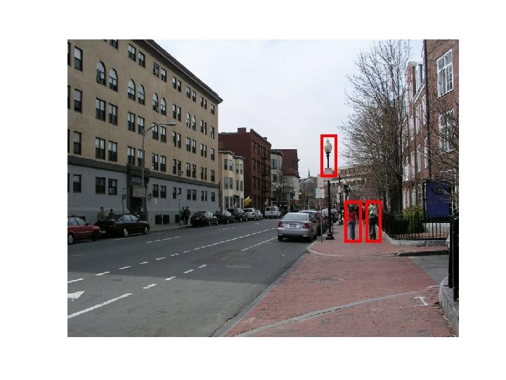
Evaluating a detector Test image (previously unseen)

First detection. . . 0. 9 ‘person’ detector predictions

Second detection. . . 0. 9 0. 6 ‘person’ detector predictions

Third detection. . . 0. 2 0. 9 0. 6 ‘person’ detector predictions

Compare to ground truth 0. 2 0. 9 0. 6 ‘person’ detector predictions ground truth ‘person’ boxes

Sort by confidence 0. 9 0. 8 . . . ✓ true positive (high overlap) 0. 6 . . . X 0. 5 . . . ✓ 0. 2 . . . ✓ 0. 1 . . . X false positive (no overlap, low overlap, or duplicate) X

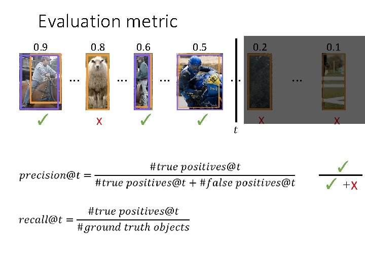
Evaluation metric 0. 9 0. 8 . . . ✓ 0. 6 . . . X 0. 5 . . . ✓ 0. 2 . . . ✓ 0. 1 . . . X X Average Precision (AP) 0% is worst 100% is best mean AP over classes (m. AP)

Pedestrians Histograms of Oriented Gradients for Human Detection, Dalal and Triggs, CVPR 2005 AP ~77% More sophisticated methods: AP ~90% (a) average gradient image over training examples (b) each “pixel” shows max positive SVM weight in the block centered on that pixel (c) same as (b) for negative SVM weights (d) test image (e) its R-HOG descriptor (f) R-HOG descriptor weighted by positive SVM weights (g) R-HOG descriptor weighted by negative SVM weights

Overview of HOG Method 1. Compute gradients in the region to be described 2. Put them in bins according to orientation 3. Group the cells into large blocks 4. Normalize each block 5. Train classifiers to decide if these are parts of a human

Details • Gradients [-1 0 1] and [-1 0 1]T were good enough filters. • Cell Histograms Each pixel within the cell casts a weighted vote for an orientation-based histogram channel based on the values found in the gradient computation. (9 channels worked) • Blocks Group the cells together into larger blocks, either R-HOG blocks (rectangular) or C-HOG blocks (circular).

More Details • Block Normalization They tried 4 different kinds of normalization. Let be the block to be normalized and e be a small constant.

Example: Dalal-Triggs pedestrian detector 1. Extract fixed-sized (64 x 128 pixel) window at each position and scale 2. Compute HOG (histogram of gradient) features within each window 3. Score the window with a linear SVM classifier 4. Perform non-maxima suppression to remove overlapping detections with lower scores Navneet Dalal and Bill Triggs, Histograms of Oriented Gradients for Human Detection, CVPR 05

Slides by Pete Barnum Navneet Dalal and Bill Triggs, Histograms of Oriented Gradients for Human Detection, CVPR 05

Outperforms centered diagonal uncentered cubic-corrected Slides by Pete Barnum Sobel Navneet Dalal and Bill Triggs, Histograms of Oriented Gradients for Human Detection, CVPR 05

• Histogram of gradient orientations Orientation: 9 bins (for unsigned angles) Histograms in 8 x 8 pixel cells • Votes weighted by magnitude • Bilinear interpolation between cells Slides by Pete Barnum Navneet Dalal and Bill Triggs, Histograms of Oriented Gradients for Human Detection, CVPR 05

Normalize with respect to surrounding cells Slides by Pete Barnum Navneet Dalal and Bill Triggs, Histograms of Oriented Gradients for Human Detection, CVPR 05

# orientations X= # features = 15 x 7 x 9 x 4 = 3780 # cells Slides by Pete Barnum # normalizations by neighboring cells Navneet Dalal and Bill Triggs, Histograms of Oriented Gradients for Human Detection, CVPR 05

Training set

pos w neg w Slides by Pete Barnum Navneet Dalal and Bill Triggs, Histograms of Oriented Gradients for Human Detection, CVPR 05

pedestrian Slides by Pete Barnum Navneet Dalal and Bill Triggs, Histograms of Oriented Gradients for Human Detection, CVPR 05

Detection examples

Deformable Parts Model • Takes the idea a little further • Instead of one rigid HOG model, we have multiple HOG models in a spatial arrangement • One root part to find first and multiple other parts in a tree structure.

The Idea Articulated parts model • • Object is configuration of parts Each part is detectable Images from Felzenszwalb

Deformable objects Images from Caltech-256 Slide Credit: Duan Tran

Deformable objects Images from D. Ramanan’s dataset Slide Credit: Duan Tran

How to model spatial relations? • Tree-shaped model

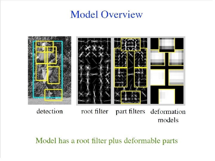
Hybrid template/parts model Detections Template Visualization Felzenszwalb et al. 2008

Pictorial Structures Model Appearance likelihood Geometry likelihood

Results for person matching 39

Results for person matching 40

BMVC 2009

2012 State-of-the-art Detector: Deformable Parts Model (DPM) Lifetime Achievement 1. Strong low-level features based on HOG 2. Efficient matching algorithms for deformable part-based models (pictorial structures) 3. Discriminative learning with latent variables (latent SVM) 42 Felzenszwalb et al. , 2008, 2010, 2011, 2012

Why did gradient-based models work? Average gradient image

Generic categories Can we detect people, chairs, horses, cars, dogs, buses, bottles, sheep …? PASCAL Visual Object Categories (VOC) dataset

Generic categories Why doesn’t this work (as well)? Can we detect people, chairs, horses, cars, dogs, buses, bottles, sheep …? PASCAL Visual Object Categories (VOC) dataset

Quiz time (Back to Girshick)

Warm up This is an average image of which object class?

Warm up pedestrian

A little harder ?

A little harder ? Hint: airplane, bicycle, bus, car, cat, chair, cow, dog, dining table

A little harder bicycle (PASCAL)

A little harder, yet ?

A little harder, yet ? Hint: white blob on a green background

A little harder, yet sheep (PASCAL)

Impossible? ?

Impossible? dog (PASCAL)

Impossible? dog (PASCAL) Why does the mean look like this? There’s no alignment between the examples! How do we combat this?

PASCAL VOC detection history mean Average Precision (m. AP) 70% 60% 50% 37% 40% 30% 23% 20% 17% 10% DPM 0% 2006 2007 DPM, HOG+ BOW 41% DPM++, Selective DPM++ 28% MKL, Search, Selective DPM++, DPM, Search MKL 2008 2009 year 2010 2011 2012 2013

Part-based models & multiple features (MKL) mean Average Precision (m. AP) 70% 60% 50% 40% 30% 20% 10% 0% 2006 nts e m ve 41% pro m i 37% ce n a DPM++, form r e p DPM++ 28% id MKL, rap 23% Selective DPM, Search 17% DPM, MKL HOG+ DPM BOW 2007 2008 2009 year 2010 41% Selective Search, DPM++, MKL 2011 2012 2013

Kitchen-sink approaches mean Average Precision (m. AP) 70% 60% increasing complexity & plateau 50% 37% 40% 30% 23% 20% 17% 10% DPM 0% 2006 2007 DPM, HOG+ BOW 41% DPM++, Selective DPM++ 28% MKL, Search, Selective DPM++, DPM, Search MKL 2008 2009 year 2010 2011 2012 2013

Region-based Convolutional Networks (R-CNNs) mean Average Precision (m. AP) 70% 62% 53% R-CNN v 2 60% 50% 37% 40% 30% 23% 20% 17% 10% DPM 0% 2006 41% 2007 DPM, HOG+ BOW 2008 41% R-CNN v 1 DPM++, Selective DPM++ 28% MKL, Search, Selective DPM++, DPM, Search MKL 2009 2010 2011 year 2012 [R-CNN. Girshick et al. CVPR 2014] 2013 2014 2015

Region-based Convolutional Networks (R-CNNs) mean Average Precision (m. AP) 70% 60% ~1 year 50% 40% ~5 years 30% 20% 10% 0% 2006 2007 2008 2009 2010 2011 year 2012 [R-CNN. Girshick et al. CVPR 2014] 2013 2014 2015

Convolutional Neural Networks • Overview

Standard Neural Networks “Fully connected”

From NNs to Convolutional NNs • Local connectivity • Shared (“tied”) weights • Multiple feature maps • Pooling

Convolutional NNs • Local connectivity compare • Each green unit is only connected to (3) neighboring blue units

Convolutional NNs • Shared (“tied”) weights

Convolutional NNs •

Convolutional NNs • Multiple feature maps • All orange units compute the same function but with a different input windows • Orange and green units compute different functions Feature map 2 (array of orange units) Feature map 1 (array of green units)

Convolutional NNs • Pooling (max, average) 1 4 0 3 4 • Pooling area: 2 units • Pooling stride: 2 units 3 • Subsamples feature maps

2 D input Pooling Convolution Image

1989 Backpropagation applied to handwritten zip code recognition , Lecun et al. , 1989

Historical perspective – 1980

Historical perspective – 1980 Hubel and Wiesel 1962 Included basic ingredients of Conv. Nets, but no supervised learning algorithm

Supervised learning – 1986 Gradient descent training with error backpropagation Early demonstration that error backpropagation can be used for supervised training of neural nets (including Conv. Nets)

Supervised learning – 1986 “T” vs. “C” problem Simple Conv. Net

Practical Conv. Nets Gradient-Based Learning Applied to Document Recognition, Lecun et al. , 1998

Demo • http: //cs. stanford. edu/people/karpathy/convnetjs/ demo/mnist. html • Conv. Net. JS by Andrej Karpathy (Ph. D. student at Stanford) Software libraries • Caffe (C++, python, matlab) • Torch 7 (C++, lua) • Theano (python)

The fall of Conv. Nets • The rise of Support Vector Machines (SVMs) • Mathematical advantages (theory, convex optimization) • Competitive performance on tasks such as digit classification • Neural nets became unpopular in the mid 1990 s

The key to SVMs • It’s all about the features HOG features SVM weights (+) (-) Histograms of Oriented Gradients for Human Detection, Dalal and Triggs, CVPR 2005

Core idea of “deep learning” • Input: the “raw” signal (image, waveform, …) • Features: hierarchy of features is learned from the raw input

• If SVMs killed neural nets, how did they come back (in computer vision)?

What’s new since the 1980 s? •

What else? Object Proposals • Sliding window based object detection Iterate over window size, aspect ratio, and location • Object proposals • Fast execution • High recall with low # of candidate boxes

The number of contours wholly enclosed by a bounding box is indicative of the likelihood of the box containing an object.

Ross’s Own System: Region CNNs

Competitive Results

Top Regions for Six Object Classes TUBITAK-EEEAG-1512

Finale • Object recognition has moved rapidly in the last 12 years to becoming very appearance based. • The HOG descriptor lead to fast recognition of specific views of generic objects, starting with pedestrians and using SVMs. • Deformable parts models extended that to allow more objects with articulated limbs, but still specific views. • CNNs have become the method of choice; they learn from huge amounts of data and can learn multiple views of each object class. 93