Object Detection Object Recognition Object Detection Object Identification

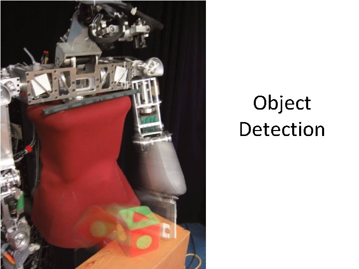
Object Detection

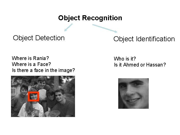
Object Recognition Object Detection Object Identification Where is Rania? Where is a Face? Is there a face in the image? Who is it? Is it Ahmed or Hassan?

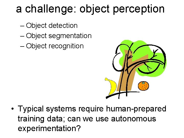
a challenge: object perception – Object detection – Object segmentation – Object recognition • Typical systems require human-prepared training data; can we use autonomous experimentation?

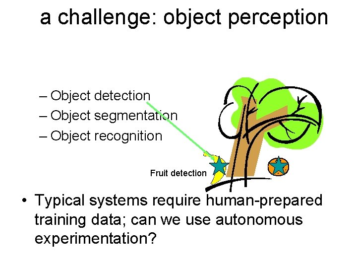
a challenge: object perception – Object detection – Object segmentation – Object recognition Fruit detection • Typical systems require human-prepared training data; can we use autonomous experimentation?

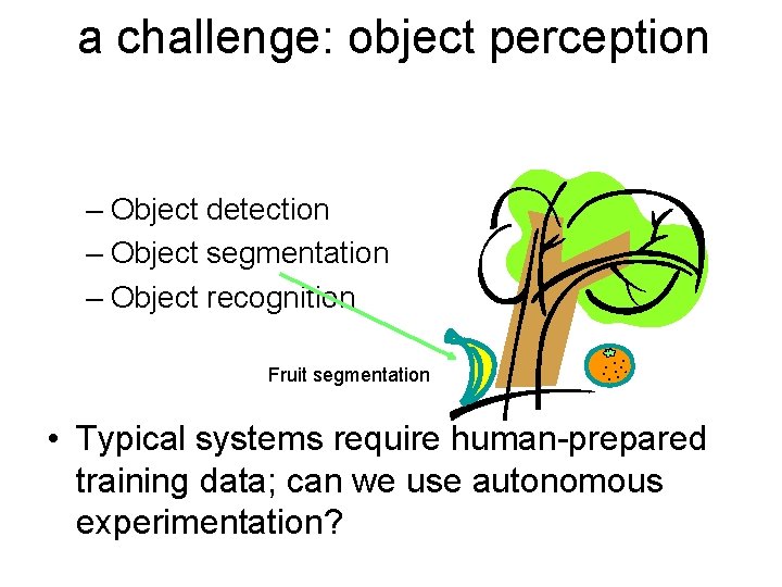
a challenge: object perception – Object detection – Object segmentation – Object recognition Fruit segmentation • Typical systems require human-prepared training data; can we use autonomous experimentation?

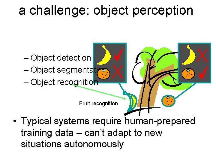
a challenge: object perception – Object detection – Object segmentation – Object recognition Fruit recognition • Typical systems require human-prepared training data – can’t adapt to new situations autonomously

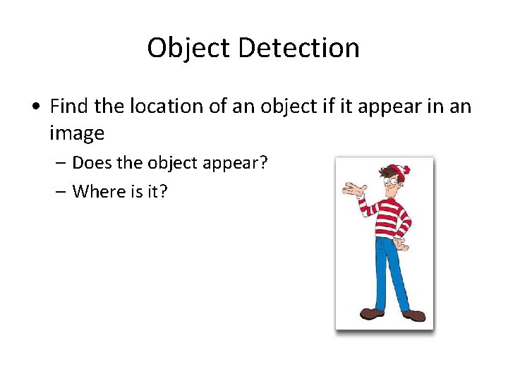
Object Detection • Find the location of an object if it appear in an image – Does the object appear? – Where is it?

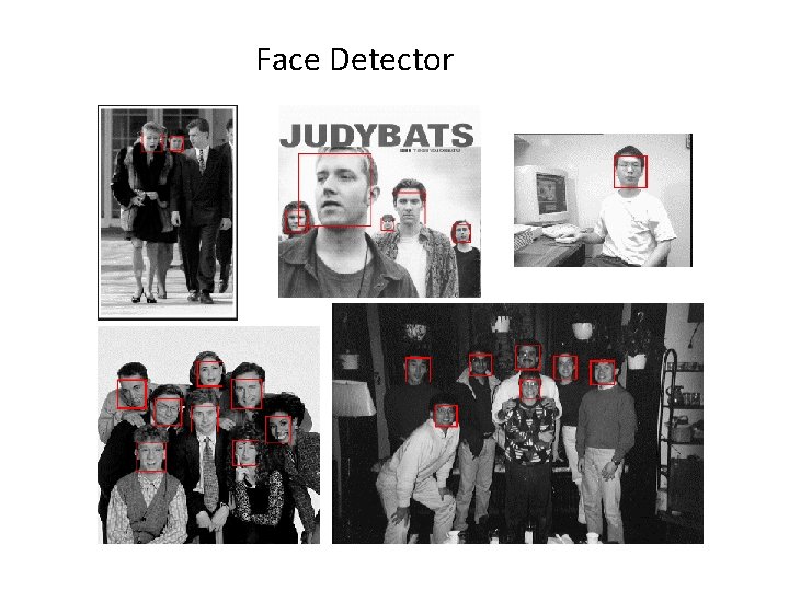
Face Detector

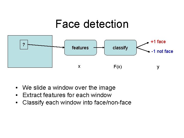
Face detection ? +1 face features x classify F(x) • We slide a window over the image • Extract features for each window • Classify each window into face/non-face -1 not face y

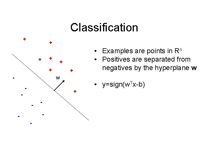
Classification + + + - • Examples are points in Rn • Positives are separated from negatives by the hyperplane w + w - • y=sign(w. Tx-b) + - - -

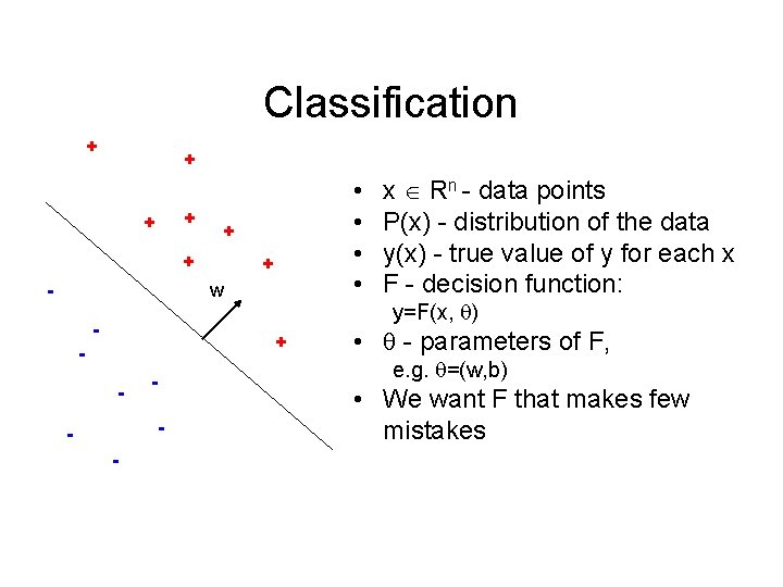
Classification + + + - • • + w - + - y=F(x, ) • - parameters of F, e. g. =(w, b) - - x Rn - data points P(x) - distribution of the data y(x) - true value of y for each x F - decision function: • We want F that makes few mistakes

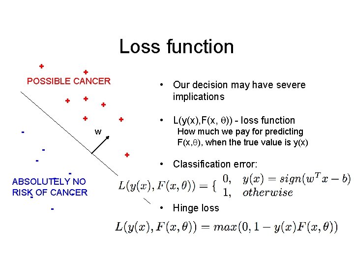
Loss function + + POSSIBLE CANCER + + - • Our decision may have severe implications • L(y(x), F(x, )) - loss function + w - How much we pay for predicting F(x, ), when the true value is y(x) + ABSOLUTELY NO RISK- OF CANCER - • Classification error: • Hinge loss

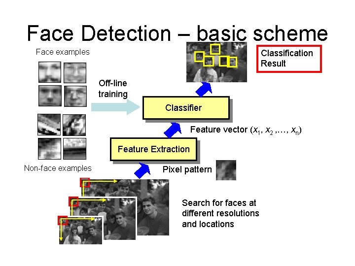
Face Detection – basic scheme Face examples Classification Result Off-line training Classifier Feature vector (x 1, x 2 , …, xn) Feature Extraction Non-face examples Pixel pattern Search for faces at different resolutions and locations

14

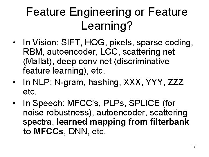
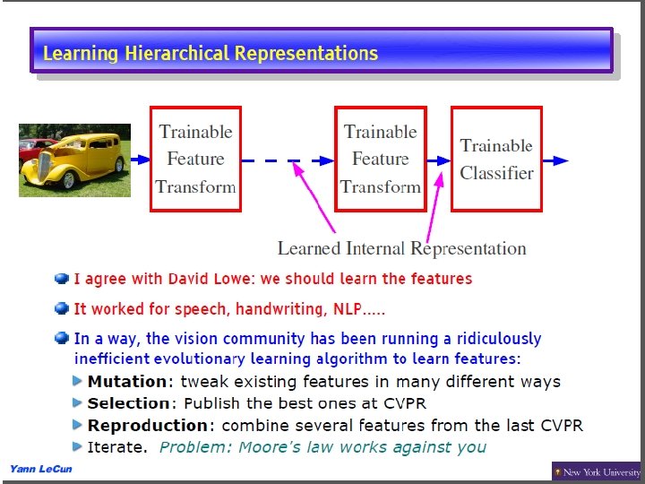
Feature Engineering or Feature Learning? • In Vision: SIFT, HOG, pixels, sparse coding, RBM, autoencoder, LCC, scattering net (Mallat), deep conv net (discriminative feature learning), etc. • In NLP: N-gram, hashing, XXX, YYY, ZZZ etc. • In Speech: MFCC’s, PLPs, SPLICE (for noise robustness), autoencoder, scattering spectra, learned mapping from filterbank to MFCCs, DNN, etc. 15

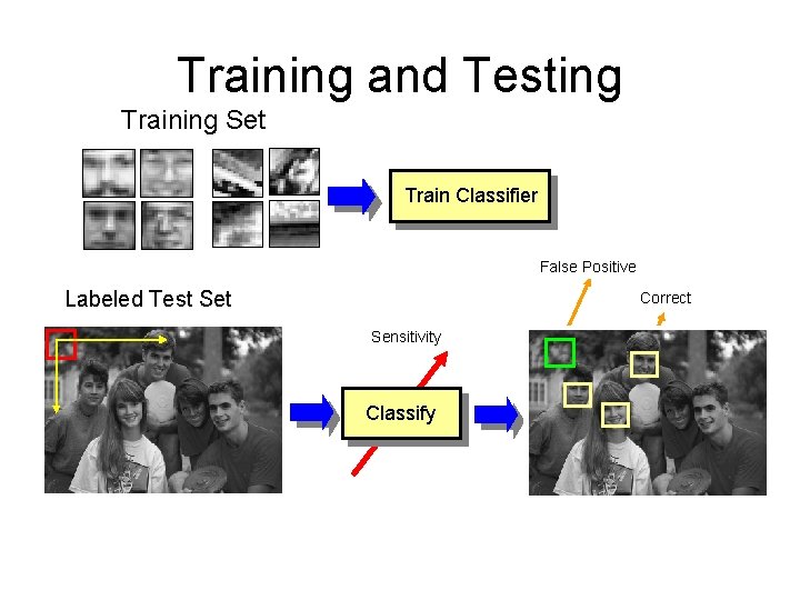
Training and Testing Training Set Train Classifier False Positive Labeled Test Set Correct Sensitivity Classify

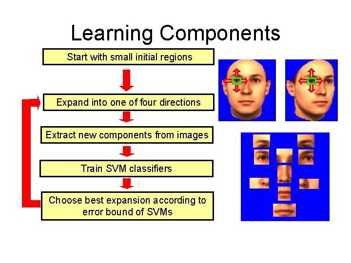
Learning Components Start with small initial regions Expand into one of four directions Extract new components from images Train SVM classifiers Choose best expansion according to error bound of SVMs

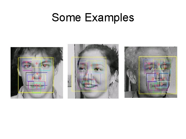
Some Examples

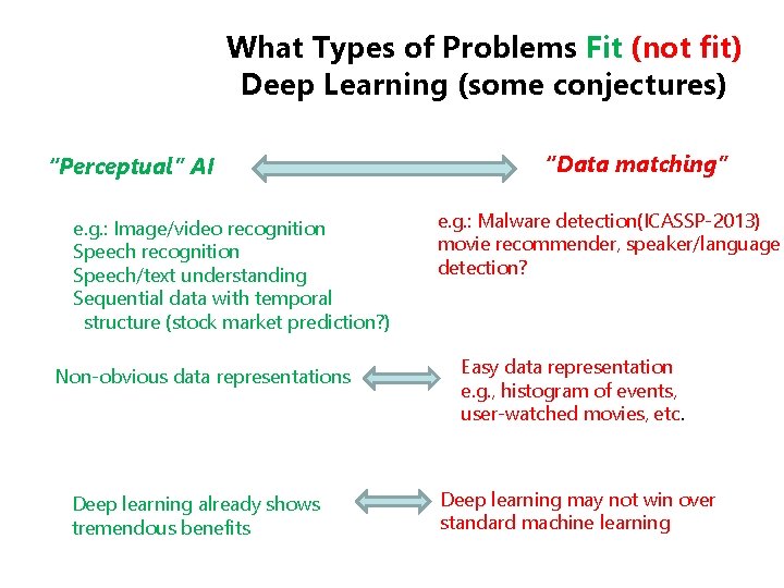
What Types of Problems Fit (not fit) Deep Learning (some conjectures) “Perceptual” AI e. g. : Image/video recognition Speech/text understanding Sequential data with temporal structure (stock market prediction? ) Non-obvious data representations Deep learning already shows tremendous benefits “Data matching” e. g. : Malware detection(ICASSP-2013) movie recommender, speaker/language detection? Easy data representation e. g. , histogram of events, user-watched movies, etc. Deep learning may not win over standard machine learning

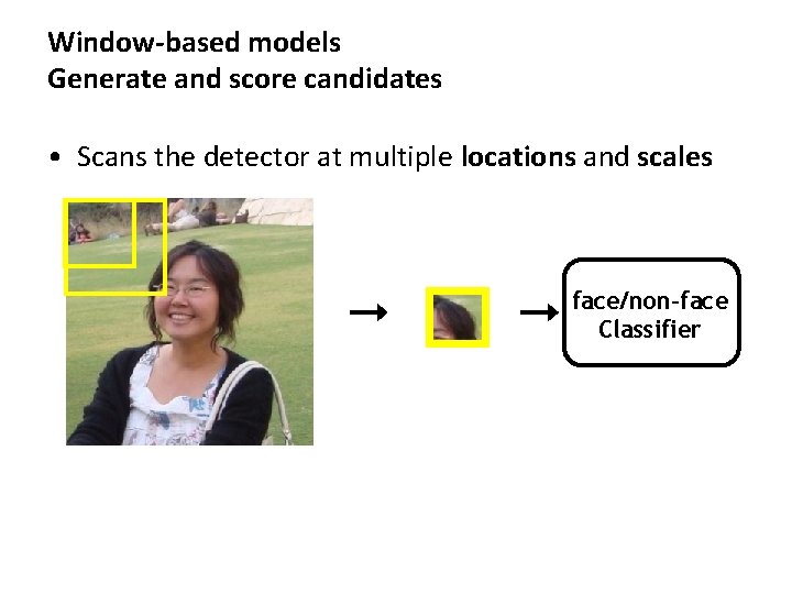
Window-based models Generate and score candidates • Scans the detector at multiple locations and scales face/non-face Classifier

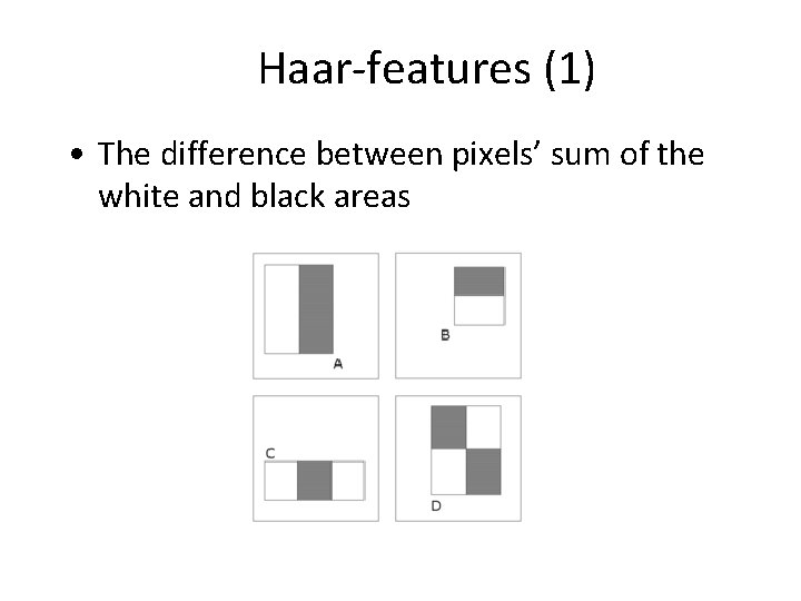
Haar-features (1) • The difference between pixels’ sum of the white and black areas

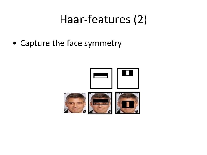
Haar-features (2) • Capture the face symmetry

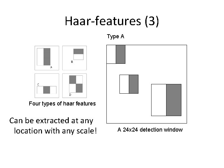
Haar-features (3) Type A Four types of haar features Can be extracted at any location with any scale! A 24 x 24 detection window

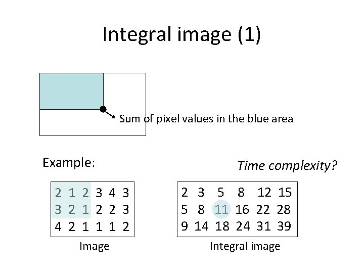
Integral image (1) Sum of pixel values in the blue area Example: 2 1 2 3 4 3 3 2 1 2 2 3 4 2 1 1 1 2 Image Time complexity? 2 3 5 8 12 15 5 8 11 16 22 28 9 14 18 24 31 39 Integral image

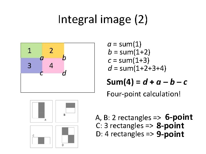
Integral image (2) 1 3 a c 2 4 b d a = sum(1) b = sum(1+2) c = sum(1+3) d = sum(1+2+3+4) Sum(4) = ? d + a – b – c Four-point calculation! A, B: 2 rectangles => 6 -point C: 3 rectangles => 8 -point D: 4 rectangles => 9 -point

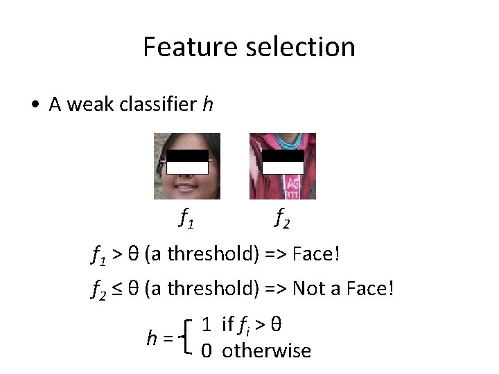
Feature selection • A weak classifier h f 1 f 2 f 1 > θ (a threshold) => Face! f 2 ≤ θ (a threshold) => Not a Face! h= 1 if fi > θ 0 otherwise

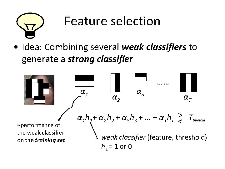
Feature selection • Idea: Combining several weak classifiers to generate a strong classifier α 1 ~performance of the weak classifier on the training set α 2 α 3 …… αT α 1 h 1+ α 2 h 2 + α 3 h 3 + … + αTh. T >< Tthresold weak classifier (feature, threshold) h 1 = 1 or 0

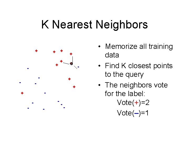
K Nearest Neighbors + + - + + +o - - + - + - - - • Memorize all training data • Find K closest points to the query • The neighbors vote for the label: Vote(+)=2 Vote(–)=1

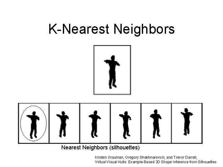
K-Nearest Neighbors (silhouettes) Kristen Grauman, Gregory Shakhnarovich, and Trevor Darrell, Virtual Visual Hulls: Example-Based 3 D Shape Inference from Silhouettes

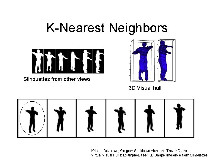
K-Nearest Neighbors Silhouettes from other views 3 D Visual hull Kristen Grauman, Gregory Shakhnarovich, and Trevor Darrell, Virtual Visual Hulls: Example-Based 3 D Shape Inference from Silhouettes

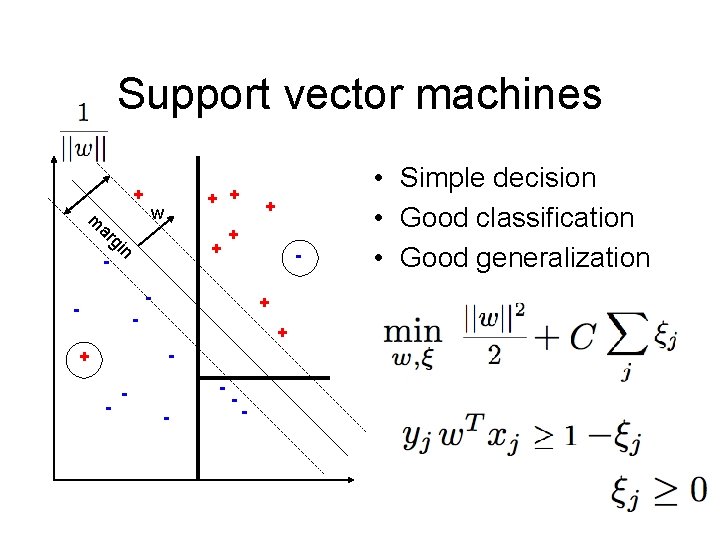
Support vector machines + m ar - gi + + w n + + + - - - + - + - - - • Simple decision • Good classification • Good generalization

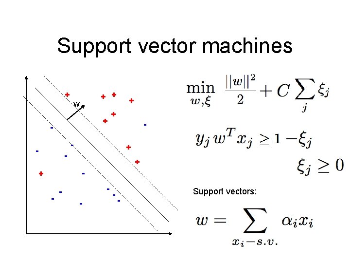
Support vector machines + + + w + - + + - - - + - + - - - Support vectors:

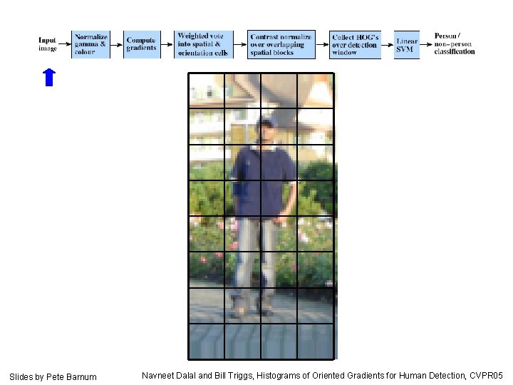
Slides by Pete Barnum Navneet Dalal and Bill Triggs, Histograms of Oriented Gradients for Human Detection, CVPR 05

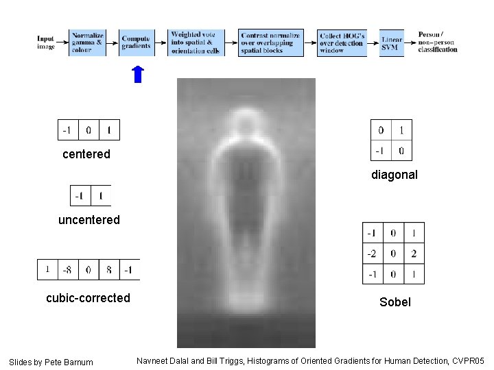
centered diagonal uncentered cubic-corrected Slides by Pete Barnum Sobel Navneet Dalal and Bill Triggs, Histograms of Oriented Gradients for Human Detection, CVPR 05

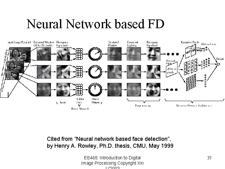
Neural Network based FD Cited from “Neural network based face detection”, by Henry A. Rowley, Ph. D. thesis, CMU, May 1999 EE 465: Introduction to Digital Image Processing Copyright Xin 35

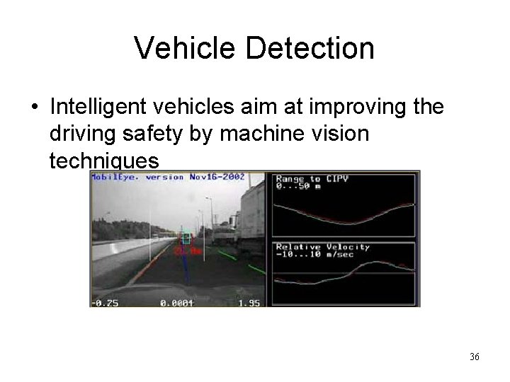
Vehicle Detection • Intelligent vehicles aim at improving the driving safety by machine vision techniques 36

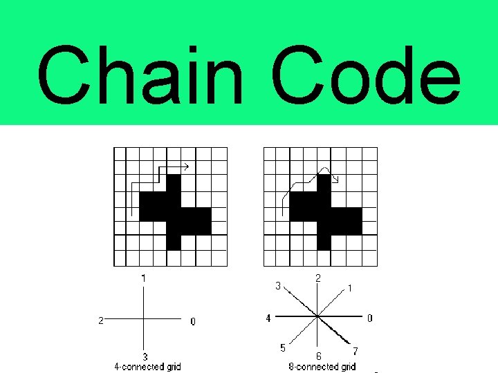
Chain Code

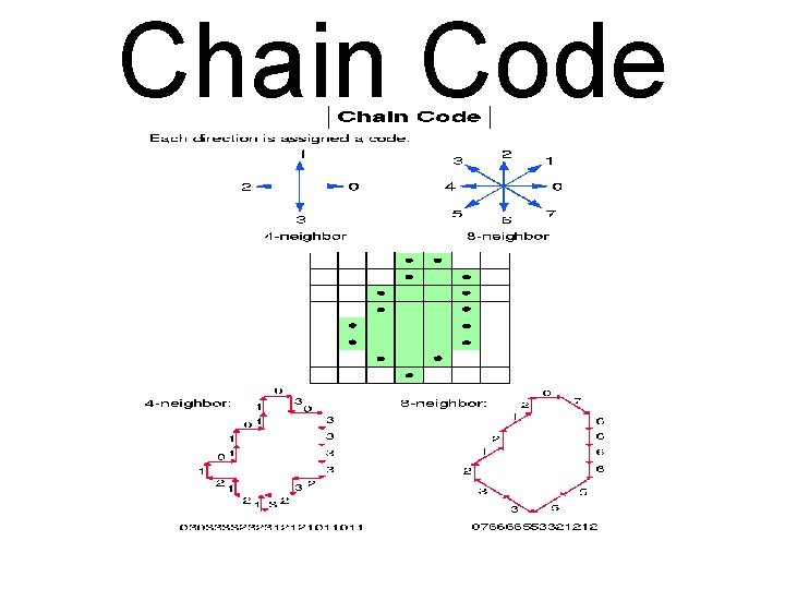
Chain Code

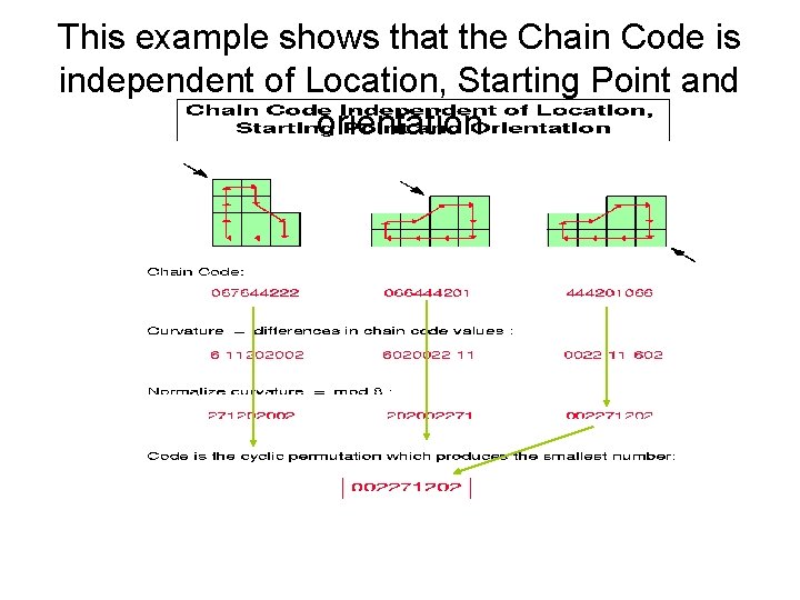
This example shows that the Chain Code is independent of Location, Starting Point and orientation

Segmentation • Segmentation – Roughly speaking, segmentation is to partition the images into meaningful parts that are relatively homogenous in certain sense

Segmentation by Fitting a Model • One view of segmentation is to group pixels (tokens, etc. ) belong together because they conform to some model – In many cases, explicit models are available, such as a line – Also in an image a line may consist of pixels that are not connected or even close to each other

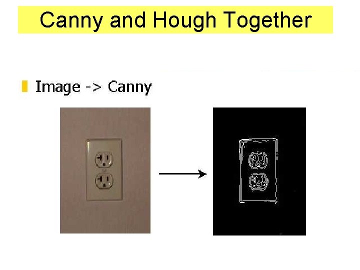
Canny and Hough Together

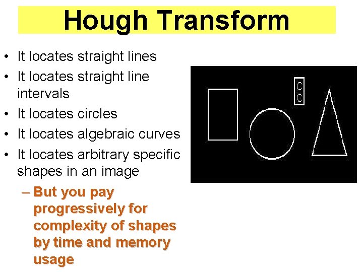
Hough Transform • It locates straight lines • It locates straight line intervals • It locates circles • It locates algebraic curves • It locates arbitrary specific shapes in an image – But you pay progressively for complexity of shapes by time and memory usage

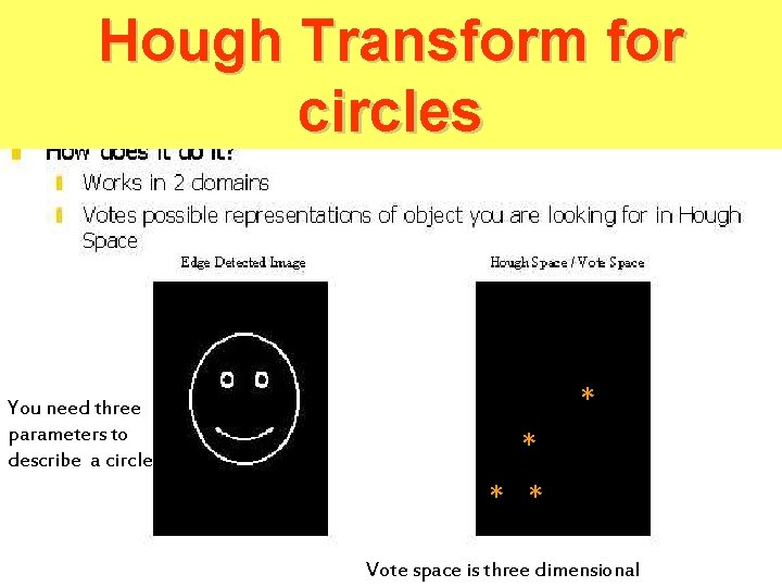
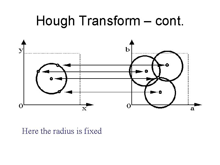
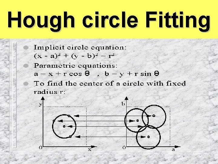
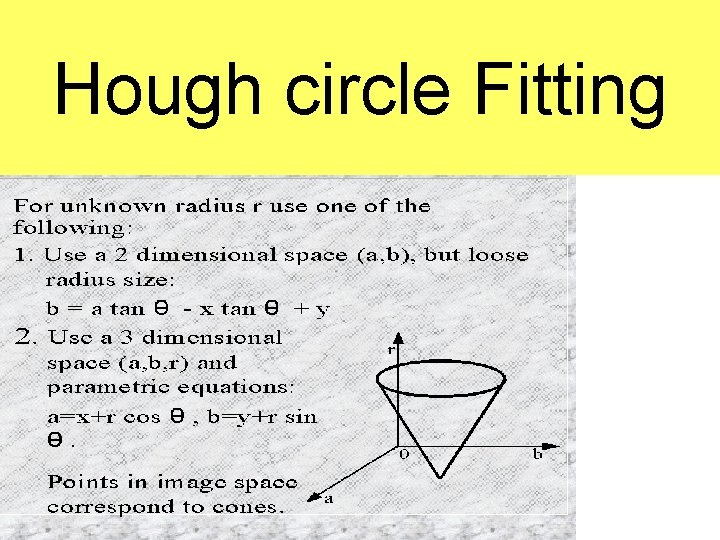
Hough Transform for circles * You need three parameters to describe a circle ** * * Vote space is three dimensional

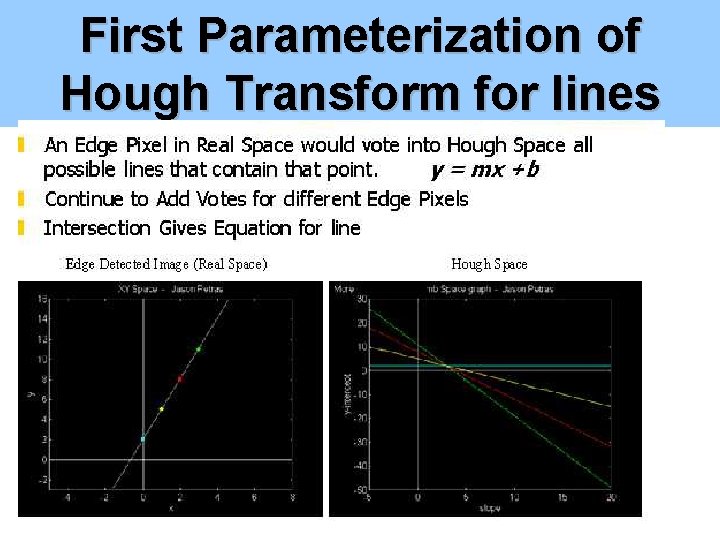
First Parameterization of Hough Transform for lines

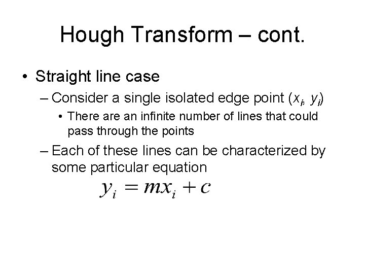
Hough Transform – cont. • Straight line case – Consider a single isolated edge point (xi, yi) • There an infinite number of lines that could pass through the points – Each of these lines can be characterized by some particular equation

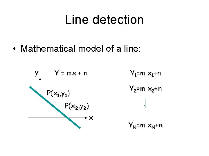
Line detection • Mathematical model of a line: y Y = mx + n Y 1=m x 1+n Y 2=m x 2+n P(x 1, y 1) P(x 2, y 2) x YN=m x. N+n

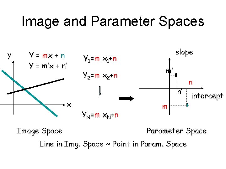
Image and Parameter Spaces y Y = mx + n Y = m’x + n’ slope Y 1= m x 1+ n Y 2=m x 2+ n m’ n’ x Image Space YN =m x N + n m n intercept Parameter Space Line in Img. Space ~ Point in Param. Space

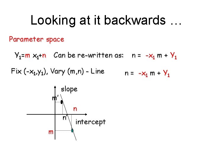
Looking at it backwards … Parameter space Y 1= m x 1+ n Can be re-written as: Fix (-x 1, y 1), Vary (m, n) - Line m’ slope n’ m n intercept n = -x 1 m + Y 1

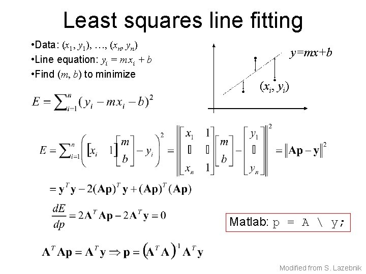
Least squares line fitting • Data: (x 1, y 1), …, (xn, yn) • Line equation: yi = m xi + b • Find (m, b) to minimize y=mx+b (xi, yi) Matlab: p = A y; Modified from S. Lazebnik

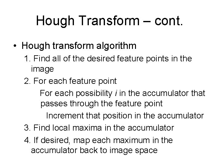
Hough Transform – cont. • Hough transform algorithm 1. Find all of the desired feature points in the image 2. For each feature point For each possibility i in the accumulator that passes through the feature point Increment that position in the accumulator 3. Find local maxima in the accumulator 4. If desired, map each maximum in the accumulator back to image space

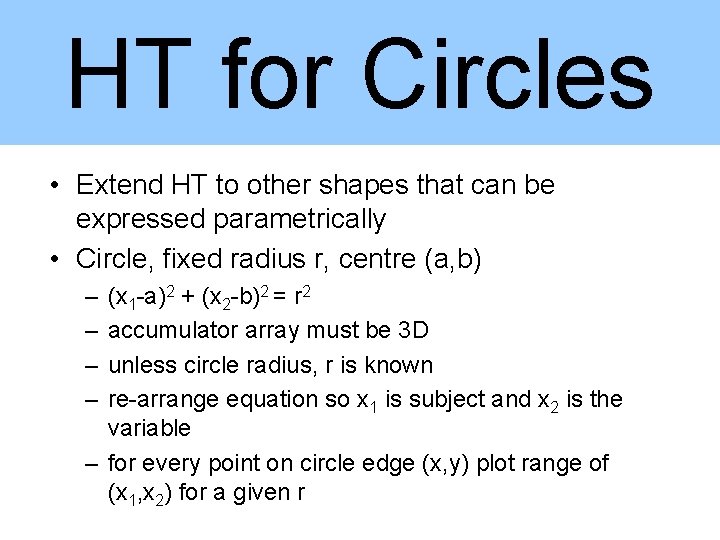
HT for Circles • Extend HT to other shapes that can be expressed parametrically • Circle, fixed radius r, centre (a, b) – – (x 1 -a)2 + (x 2 -b)2 = r 2 accumulator array must be 3 D unless circle radius, r is known re-arrange equation so x 1 is subject and x 2 is the variable – for every point on circle edge (x, y) plot range of (x 1, x 2) for a given r

Hough Transform – cont. Here the radius is fixed

Hough circle Fitting

Hough circle Fitting