Object Recognizing Object Classes Individual Recognition Object parts

Object Recognizing

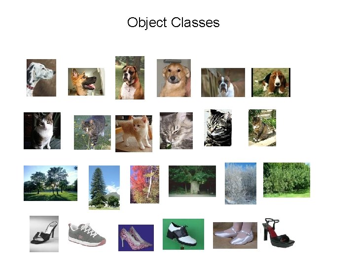
Object Classes

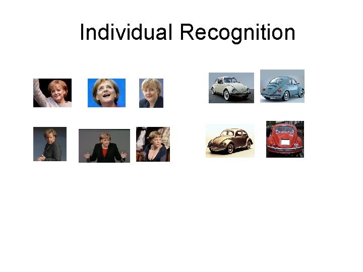
Individual Recognition

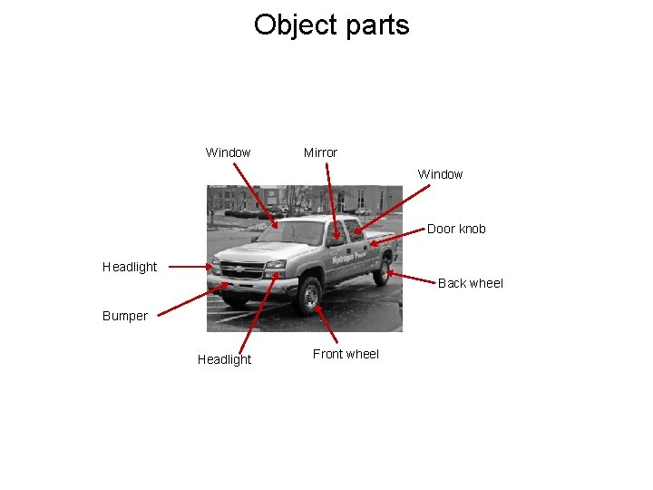
Object parts Window Mirror Window Door knob Headlight Back wheel Bumper Headlight Front wheel

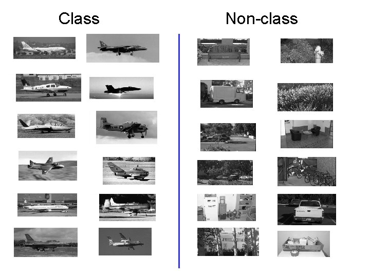
Class Non-class

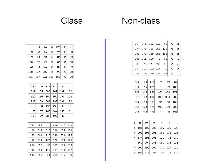
Class Non-class

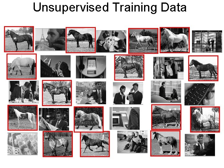
Unsupervised Training Data

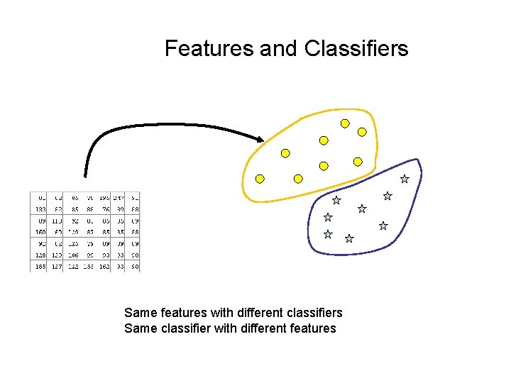
Features and Classifiers Same features with different classifiers Same classifier with different features

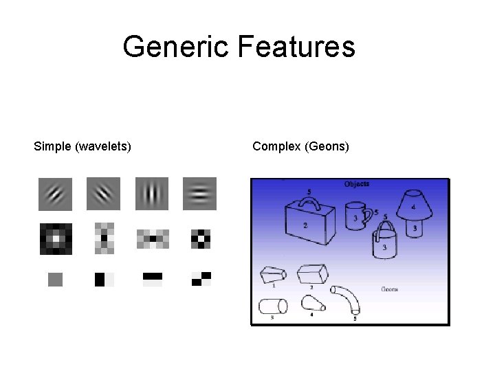
Generic Features Simple (wavelets) Complex (Geons)

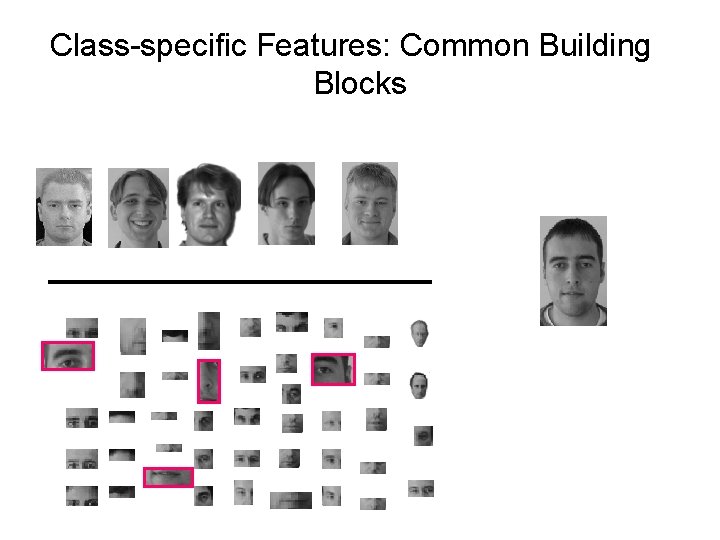
Class-specific Features: Common Building Blocks

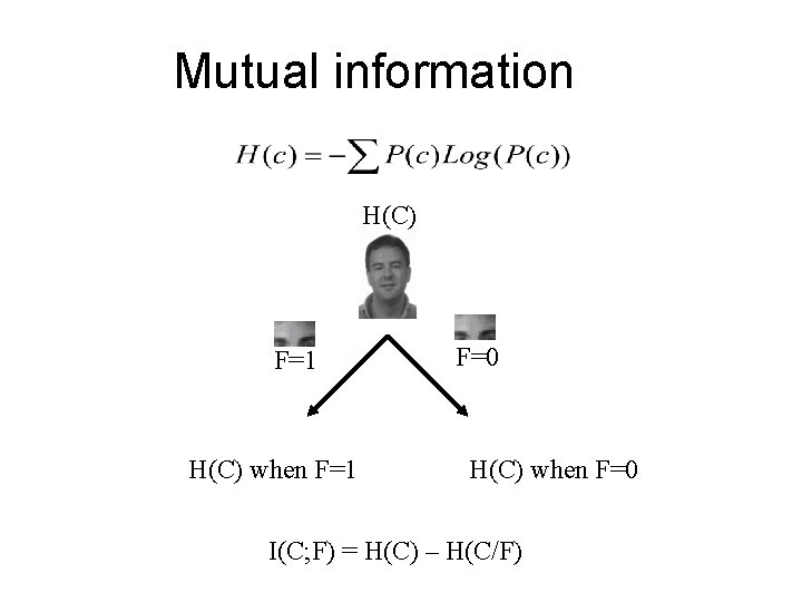
Mutual information H(C) F=1 H(C) when F=1 F=0 H(C) when F=0 I(C; F) = H(C) – H(C/F)

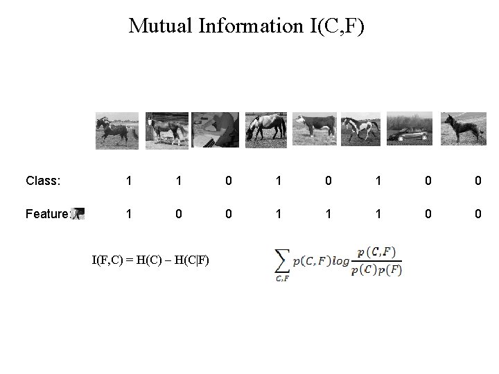
Mutual Information I(C, F) Class: 1 1 0 1 0 0 Feature: 1 0 0 1 1 1 0 0 I(F, C) = H(C) – H(C|F)

Optimal classification features • Theoretically: maximizing delivered information minimizes classification error • In practice: informative object components can be identified in training images

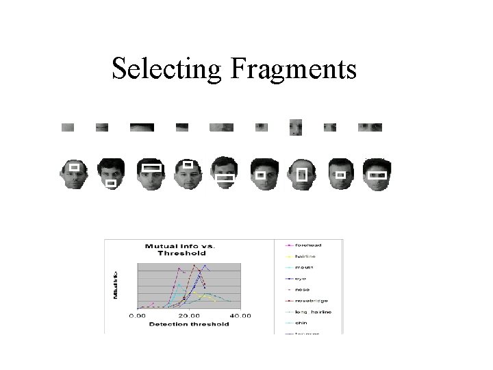
Selecting Fragments

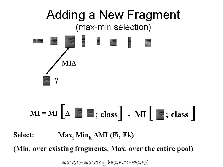
Adding a New Fragment (max-min selection) MIΔ ? MI = MI Select: [Δ ; class ] - MI [ ; class ] Maxi Mink ΔMI (Fi, Fk) (Min. over existing fragments, Max. over the entire pool)

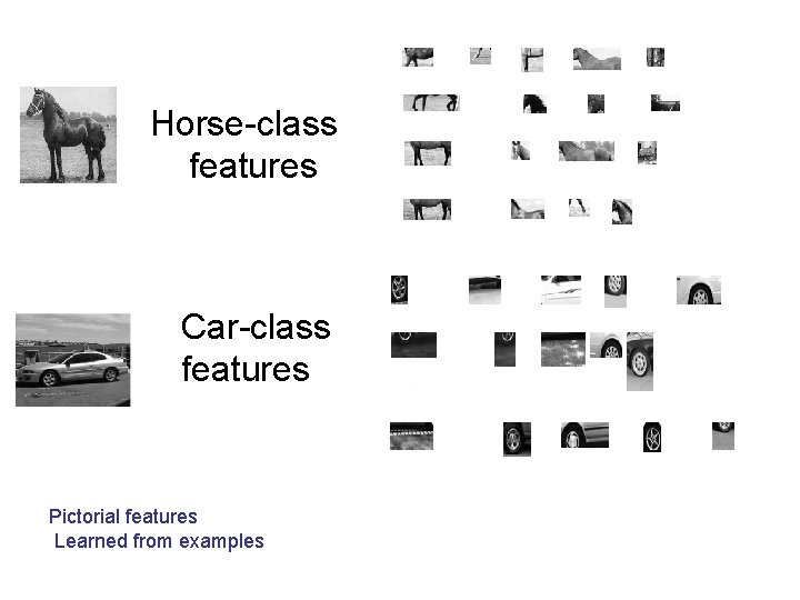
Horse-class features Car-class features Pictorial features Learned from examples

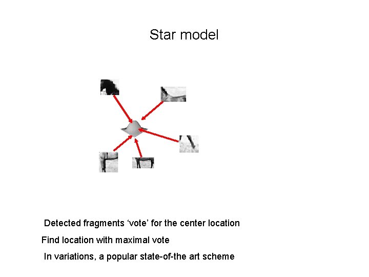
Star model Detected fragments ‘vote’ for the center location Find location with maximal vote In variations, a popular state-of-the art scheme

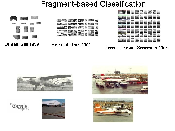
Fragment-based Classification Ullman, Sali 1999 Agarwal, Roth 2002 Fergus, Perona, Zisserman 2003

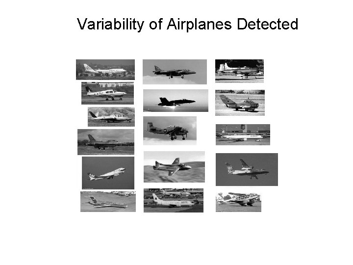
Variability of Airplanes Detected

Recognition Features in the Brain

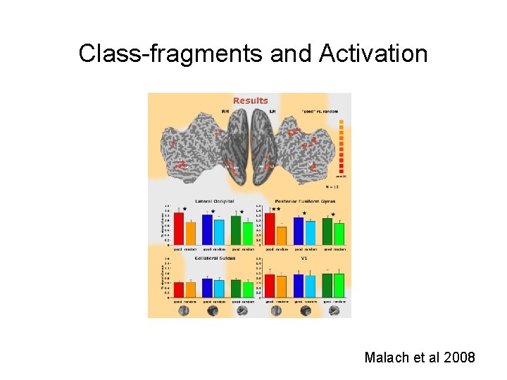
Class-fragments and Activation Malach et al 2008

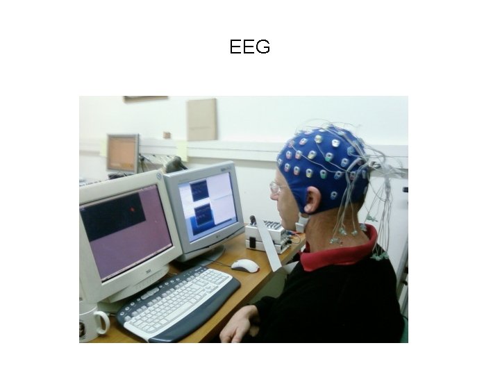
EEG

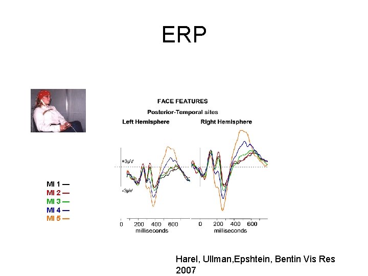
ERP MI 1 — MI 2 — MI 3 — MI 4 — MI 5 — Harel, Ullman, Epshtein, Bentin Vis Res 2007

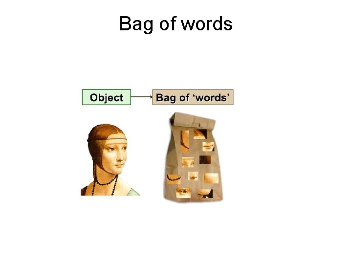
Bag of words

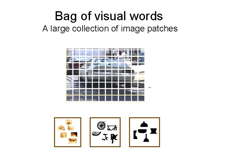
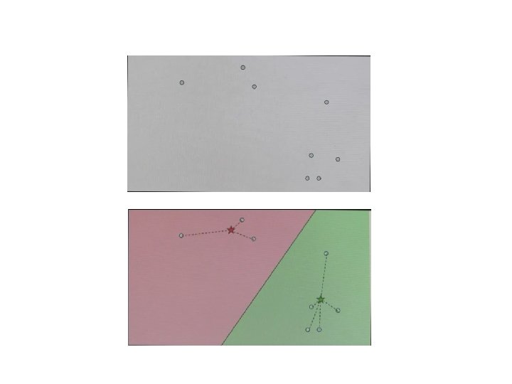
Bag of visual words A large collection of image patches –

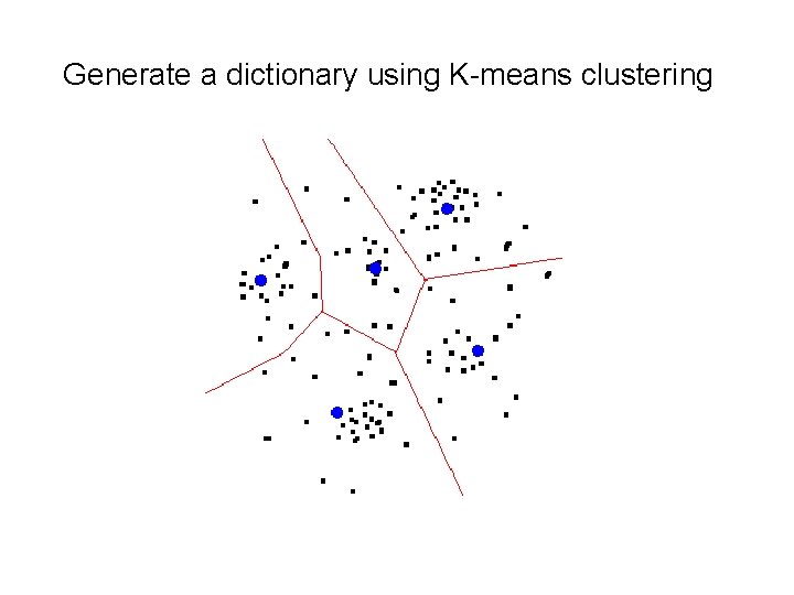
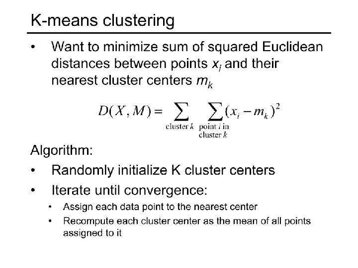
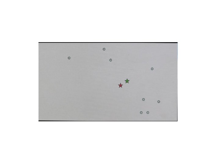
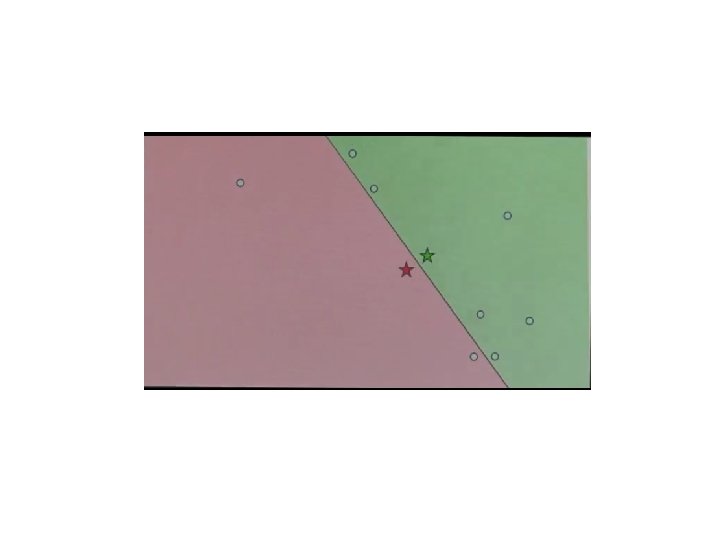
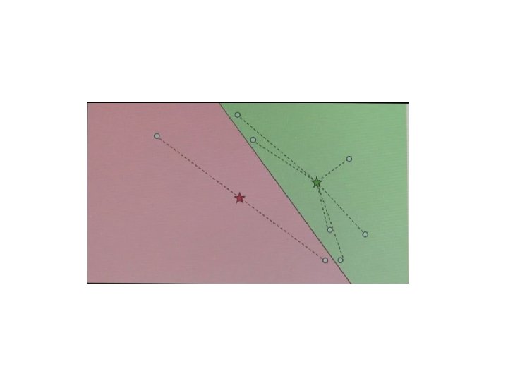
Generate a dictionary using K-means clustering

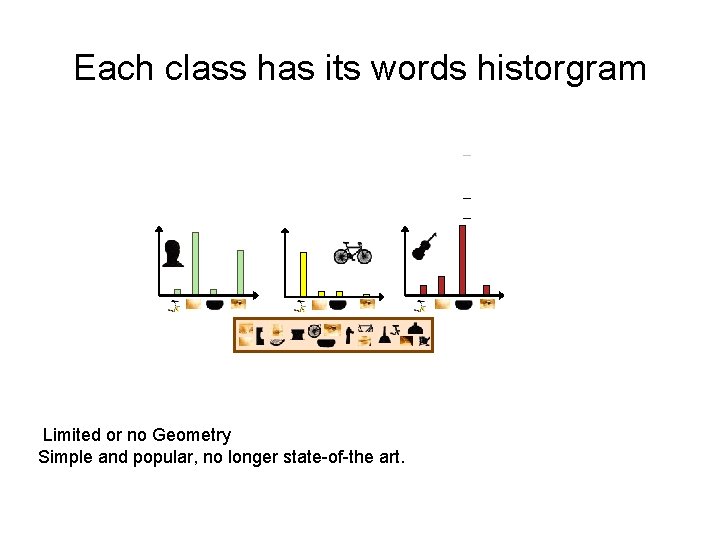
Each class has its words historgram – – – Limited or no Geometry Simple and popular, no longer state-of-the art.

Classifiers

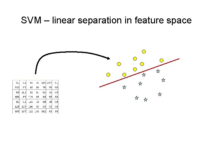
SVM – linear separation in feature space

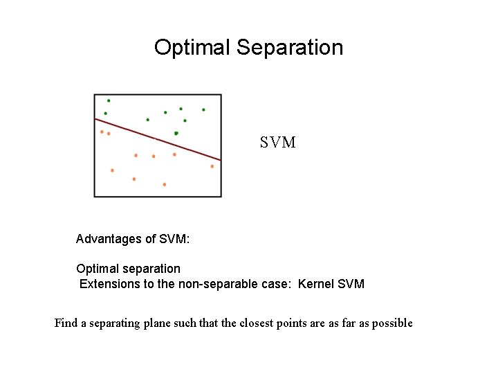
Optimal Separation SVM Advantages of SVM: Optimal separation Extensions to the non-separable case: Kernel SVM Find a separating plane such that the closest points are as far as possible

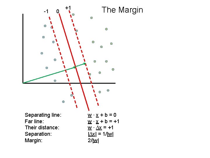
-1 0 Separating line: Far line: Their distance: Separation: Margin: +1 The Margin w∙x+b=0 w ∙ x + b = +1 w ∙ ∆x = +1 |∆x| = 1/|w| 2/|w|

Max Margin Classification The examples are vectors xi The labels yi are +1 for class, -1 for non-class (Equivalently, usually used How to solve such constraint optimization?

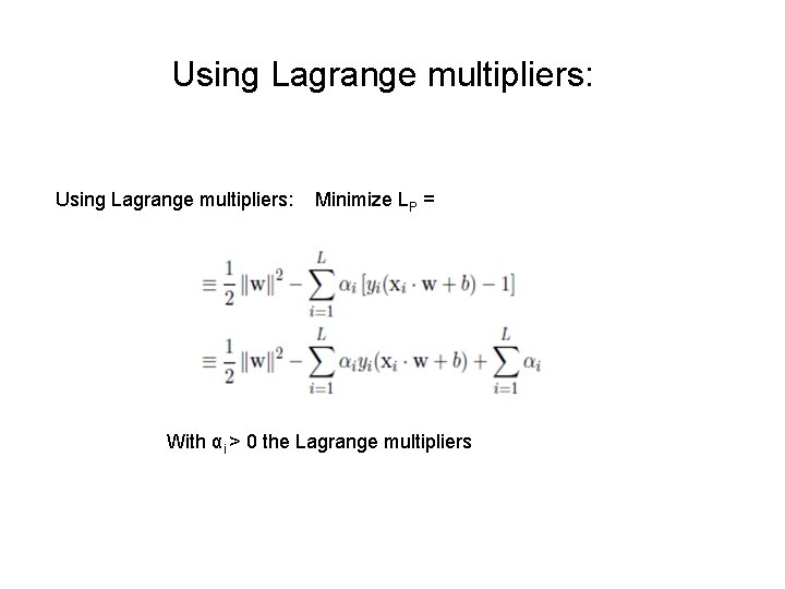
Using Lagrange multipliers: Minimize LP = With αi > 0 the Lagrange multipliers

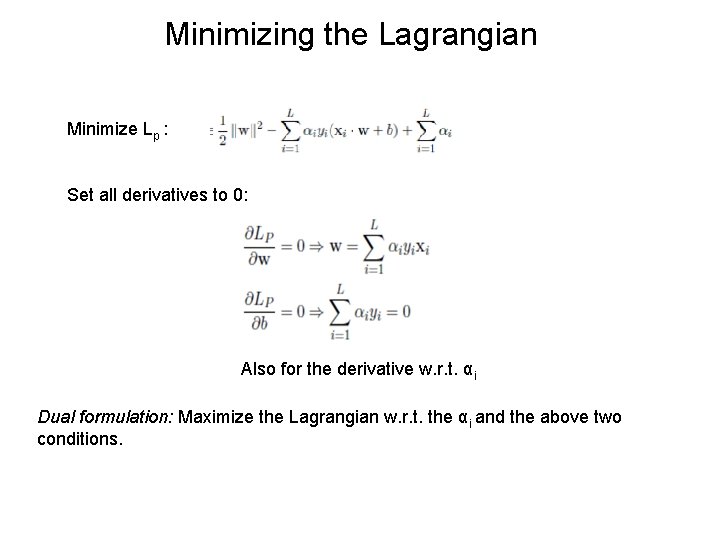
Minimizing the Lagrangian Minimize Lp : Set all derivatives to 0: Also for the derivative w. r. t. αi Dual formulation: Maximize the Lagrangian w. r. t. the αi and the above two conditions.

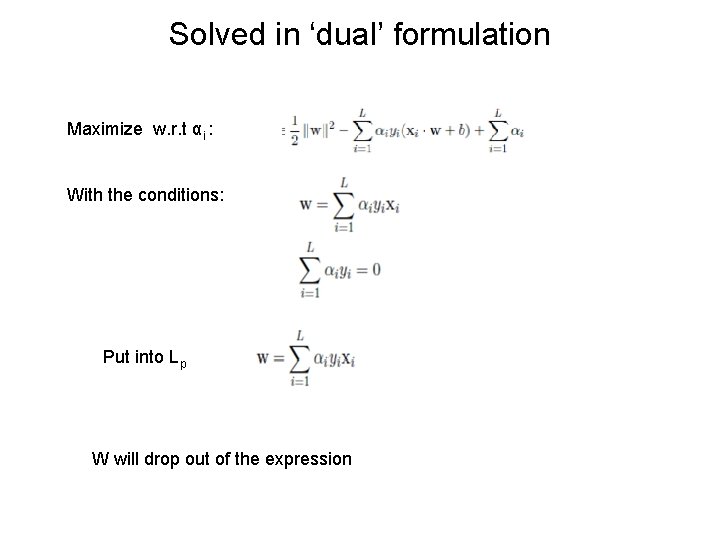
Solved in ‘dual’ formulation Maximize w. r. t αi : With the conditions: Put into Lp W will drop out of the expression

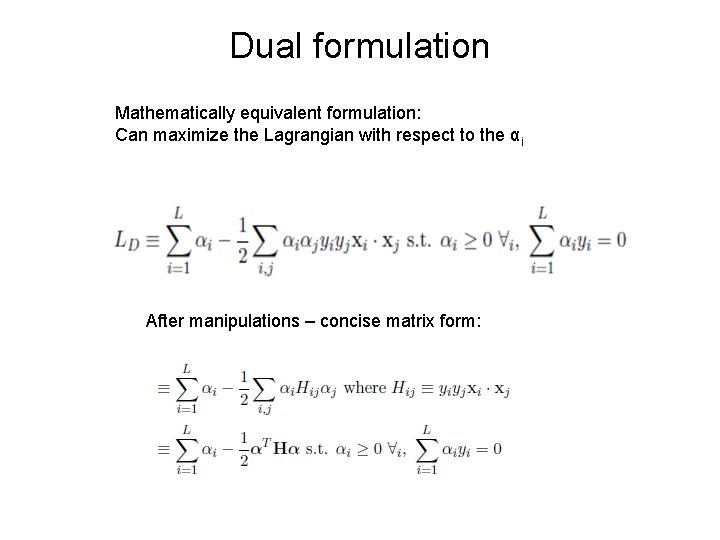
Dual formulation Mathematically equivalent formulation: Can maximize the Lagrangian with respect to the αi After manipulations – concise matrix form:

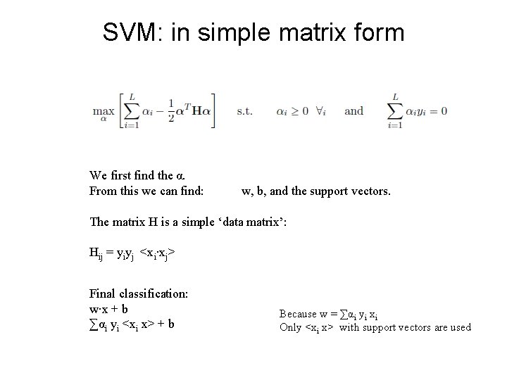
SVM: in simple matrix form We first find the α. From this we can find: w, b, and the support vectors. The matrix H is a simple ‘data matrix’: Hij = yiyj <xi∙xj> Final classification: w∙x + b ∑αi yi <xi x> + b Because w = ∑αi yi xi Only <xi x> with support vectors are used

DPM Felzenszwalb • Felzenszwalb, Mc. Allester, Ramanan CVPR 2008. A Discriminatively Trained, Multiscale, Deformable Part Model • Many implementation details, will describe the main points.

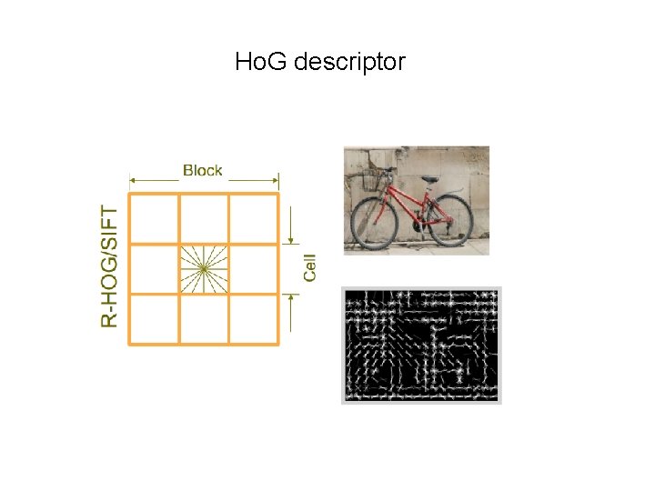
Ho. G descriptor

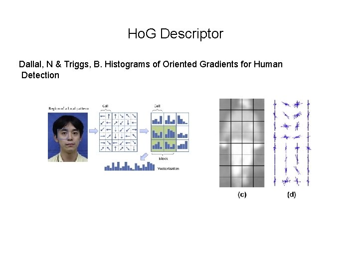
Ho. G Descriptor Dallal, N & Triggs, B. Histograms of Oriented Gradients for Human Detection

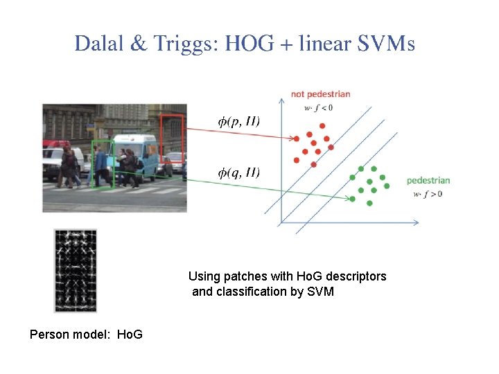
Using patches with Ho. G descriptors and classification by SVM Person model: Ho. G

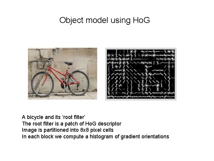
Object model using Ho. G A bicycle and its ‘root filter’ The root filter is a patch of Ho. G descriptor Image is partitioned into 8 x 8 pixel cells In each block we compute a histogram of gradient orientations

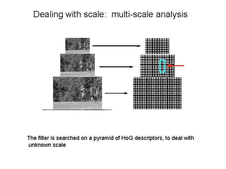
Dealing with scale: multi-scale analysis The filter is searched on a pyramid of Ho. G descriptors, to deal with unknown scale

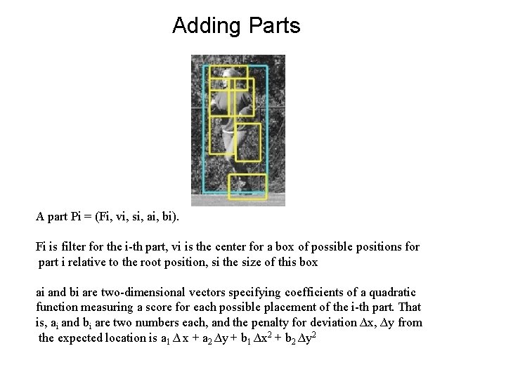
Adding Parts A part Pi = (Fi, vi, si, ai, bi). Fi is filter for the i-th part, vi is the center for a box of possible positions for part i relative to the root position, si the size of this box ai and bi are two-dimensional vectors specifying coefficients of a quadratic function measuring a score for each possible placement of the i-th part. That is, ai and bi are two numbers each, and the penalty for deviation ∆x, ∆y from the expected location is a 1 ∆ x + a 2 ∆y + b 1 ∆x 2 + b 2 ∆y 2

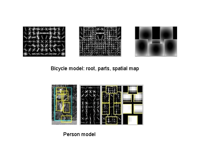
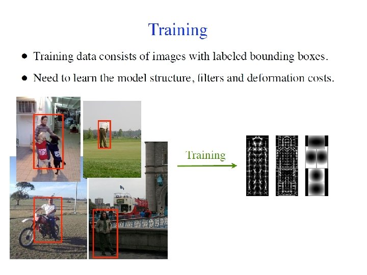
Bicycle model: root, parts, spatial map Person model

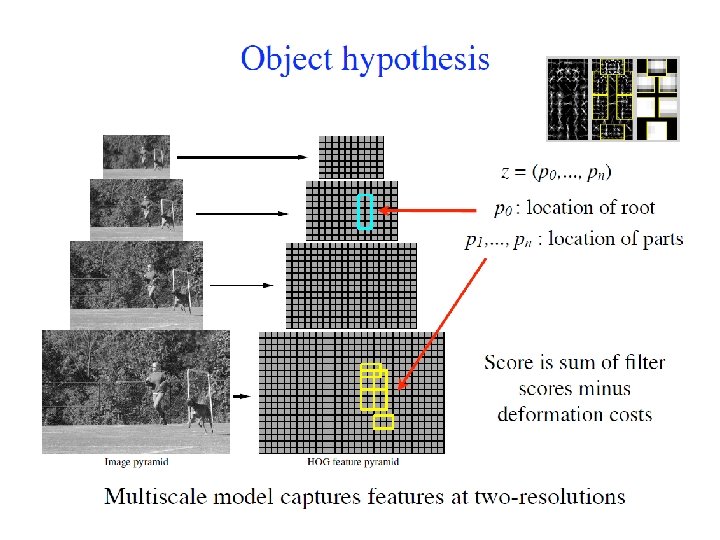
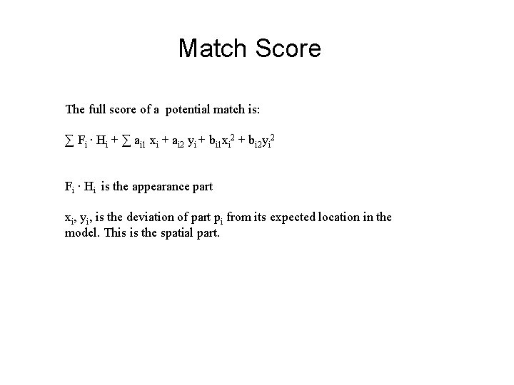
Match Score The full score of a potential match is: ∑ Fi ∙ Hi + ∑ ai 1 xi + ai 2 yi + bi 1 xi 2 + bi 2 yi 2 Fi ∙ Hi is the appearance part xi, yi, is the deviation of part pi from its expected location in the model. This is the spatial part.

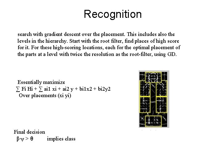
Recognition search with gradient descent over the placement. This includes also the levels in the hierarchy. Start with the root filter, find places of high score for it. For these high-scoring locations, each for the optimal placement of the parts at a level with twice the resolution as the root-filter, using GD. Essentially maximize ∑ Fi Hi + ∑ ai 1 xi + ai 2 y + bi 1 x 2 + bi 2 y 2 Over placements (xi yi) Final decision β∙ψ > θ implies class

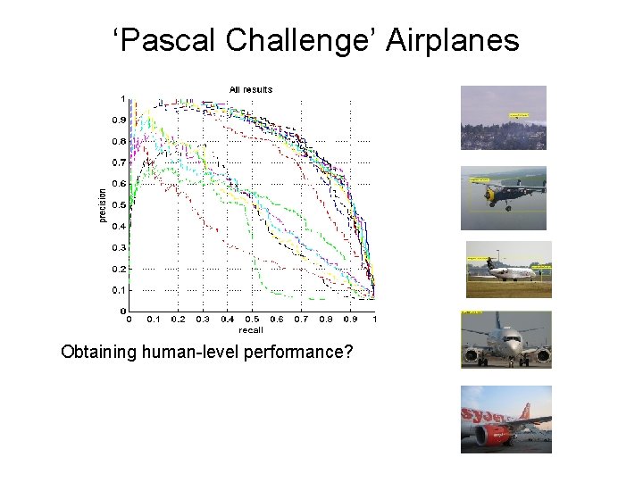
‘Pascal Challenge’ Airplanes Obtaining human-level performance?

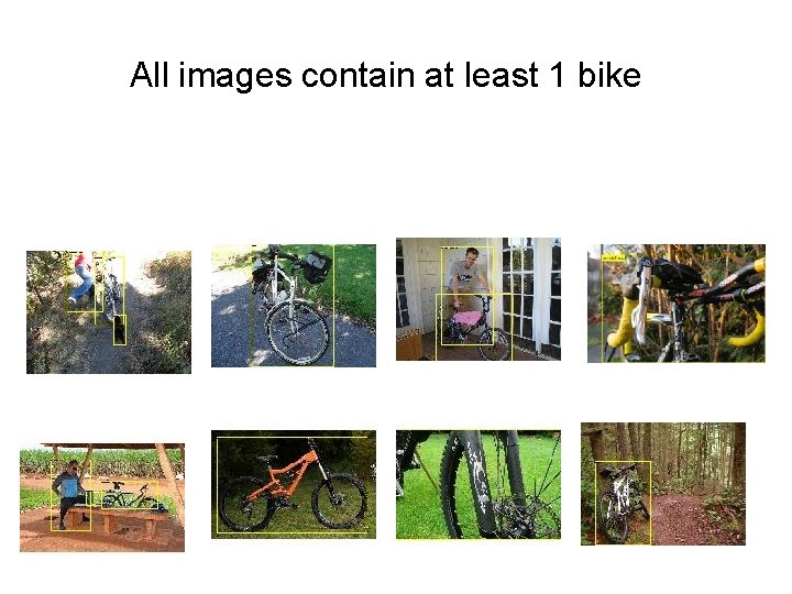
All images contain at least 1 bike

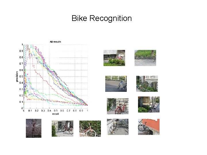
Bike Recognition