Rich Feature Hierarchies for Accurate Object Detection and

Rich Feature Hierarchies for Accurate Object Detection and Semantic Segmentation Ross Girshick, Jeff Donahue, Trevor Darrell, Jitendra Malik

PASCAL VOC detection history 37% 23% 17% DPM, DPM HOG+BOW 41% DPM++, Selective DPM++ MKL, Search, 28% Selective DPM++, DPM, Search MKL VOC’ 07 VOC’ 08 VOC’ 09 VOC’ 10 VOC’ 11 VOC’ 12 PASCAL VOC challenge dataset [Source: http: //pascallin. ecs. soton. ac. uk/challenges/VOC/voc 20{07, 08, 09, 10, 11, 12}/results/index. html]

A rapid rise in performance 37% 23% 17% DPM, DPM HOG+BOW 41% DPM++, Selective DPM++ MKL, Search, 28% Selective DPM++, DPM, Search MKL VOC’ 07 VOC’ 08 VOC’ 09 VOC’ 10 VOC’ 11 VOC’ 12 PASCAL VOC challenge dataset [Source: http: //pascallin. ecs. soton. ac. uk/challenges/VOC/voc 20{07, 08, 09, 10, 11, 12}/results/index. html]

Complexity and the plateau & increasing complexity 37% 23% 17% DPM, DPM HOG+BOW 41% DPM++, Selective DPM++ MKL, Search, 28% Selective DPM++, DPM, Search MKL VOC’ 07 VOC’ 08 VOC’ 09 VOC’ 10 VOC’ 11 VOC’ 12 PASCAL VOC challenge dataset [Source: http: //pascallin. ecs. soton. ac. uk/challenges/VOC/voc 20{07, 08, 09, 10, 11, 12}/results/index. html]

SIFT, HOG, LBP, . . . Seg. DPM (2013) Regionlets (2013) DPM++, Selective (2013) DPM++ MKL, Search, Selective DPM++, DPM, Search MKL DPM, DPM HOG+BOW VOC’ 07 VOC’ 08 VOC’ 09 VOC’ 10 VOC’ 11 VOC’ 12 PASCAL VOC challenge dataset [Regionlets. Wang et al. [Seg. DPM. Fidler et al. ICCV’ 13] CVPR’ 13]

R-CNN: Regions with CNN features R-CNN 58. 5% R-CNN 53. 7% R-CNN 53. 3% VOC’ 07 VOC’ 08 VOC’ 09 VOC’ 10 VOC’ 11 VOC’ 12 PASCAL VOC challenge dataset

Feature learning with CNNs Fukushima 1980 Neocognitron

Feature learning with CNNs Fukushima 1980 Neocognitron Rumelhart, Hinton, Williams 1986 “T” versus “C” problem

Feature learning with CNNs Fukushima 1980 Neocognitron Rumelhart, Hinton, Williams 1986 “T” versus “C” problem Le. Cun et al. 1989 -1998 Handwritten digit reading / OCR

Feature learning with CNNs Fukushima 1980 Neocognitron Rumelhart, Hinton, Williams 1986 “T” versus “C” problem Le. Cun et al. 1989 -1998. . . Handwritten digit reading / OCR Krizhevksy, Sutskever, Hinton 2012 Image. Net classification breakthrough “Super. Vision” CNN

CNNs for object detection Vaillant, Monrocq, Le. Cun 1994 Multi-scale face detection Le. Cun, Huang, Bottou 2004 NORB dataset Cireşan et al. 2013 Mitosis detection Sermanet et al. 2013 Pedestrian detection Szegedy, Toshev, Erhan 2013 PASCAL detection (VOC’ 07 m. AP 30. 5

Can we break through the PASCAL plateau with feature learning?

R-CNN: Regions with CNN features Input Extract region image proposals (~2 k / image) Compute CNN features Classify regions (linear SVM)

R-CNN at test time: Step 1 Input Extract region image proposals (~2 k / image) Proposal-method agnostic, many choices - Selective Search [van de Sande, Uijlings et al. ] (Used in this work) - Objectness [Alexe et al. ] - Category independent object proposals [Endres & Hoiem] - CPMC [Carreira & Sminchisescu] Active area, at this CVPR - BING [Ming et al. ] – fast - MCG [Arbelaez et al. ] – high-quality segmentation

R-CNN at test time: Step 2 Input Extract region image proposals (~2 k / image) Compute CNN features

R-CNN at test time: Step 2 Input Extract region image proposals (~2 k / image) Compute CNN features Dilate proposal

R-CNN at test time: Step 2 Input Extract region image proposals (~2 k / image) a. Crop Compute CNN features

R-CNN at test time: Step 2 Input Extract region image proposals (~2 k / image) Compute CNN features 227 x 227 a. Crop b. Scale (anisotropic)

R-CNN at test time: Step 2 Input Extract region image proposals (~2 k / image) Compute CNN features c. Forward propagate. Crop b. Scale (anisotropic) Output: “fc 7” features

R-CNN at test time: Step 3 Input Extract region image proposals (~2 k / image) Compute CNN features person? 1. 6 . . . horse? -0. 3 . . . 4096 -dimensional linear classifiers d proposal fc 7 feature vector (SVM or softmax) Classify regions

Step 4: Object proposal refinement Linear regression on CNN features Original proposal Predicted object bounding box Bounding-box regression

Bounding-box regression w h Δw × w + w (x, y) (Δx × w + x, Δy × h + h) Δh × h + h original predicted

R-CNN results on PASCAL DPM v 5 (Girshick et al. 2011) VOC 2007 VOC 2010 33. 7% 29. 6% UVA sel. search (Uijlings et al. 2013) Regionlets (Wang et al. 2013) 35. 1% 41. 7% Seg. DPM (Fidler et al. 2013) R-CNN 40. 4% 54. 2% Reference systems R-CNN + bbox regression 39. 7% 58. 5% 50. 2% 53. 7% metric: mean average precision (higher is better)

R-CNN results on PASCAL DPM v 5 (Girshick et al. 2011) VOC 2007 VOC 2010 33. 7% 29. 6% UVA sel. search (Uijlings et al. 2013) Regionlets (Wang et al. 2013) 35. 1% 41. 7% Seg. DPM (Fidler et al. 2013) 39. 7% 40. 4% R-CNN 54. 2% 50. 2% R-CNN + bbox regression 58. 5% 53. 7% metric: mean average precision (higher is better)

Top bicycle FPs (AP = 72. 8%)

False positive #15

False positive #15 (zoom) Unannotated bicycle

False positive #15 1949 French comedy by Jacques Tati

False positive type distribution Loc = localization Oth = other / dissimilar classes Sim = similar classes BG = background Analysis software: D. Hoiem, Y. Chodpathumwan, and Q. Dai. Diagnosing Error in Object Detectors. ECCV, 2012.

Training R-CNN Bounding-box labeled detection data is scarce Key insight: Use supervised pre-training on a datarich auxiliary task and transfer to detection

Image. Net LSVR Challenge – Image classification (not detection) – 1000 classes (vs. 20) – 1. 2 million training labels (vs. 25 k) bus anywhere? [Deng et al. CVPR’ 09]

ILSVRC 2012 winner “Super. Vision” Convolutional Neural Network (CNN) input 5 convolutional layers fully connected Image. Net Classification with Deep Convolutional Neural Networks. Krizhevsky, Sutskever, Hinton. NIPS 2012.

Impressive Image. Net results! 1000 -way image classification Top-5 error Fisher Vectors (ISI) 26. 2% 5 Super. Vision 16. 4% CNNs now: ~12% 7 Super. Vision 15. 3% metric: classification error rate (lower is better) CNNs But. . . does it generalize to other datasets and tasks? [See also: De. CAF. Donahue et al. , ICML 2014. ] Spirited debate at ECCV 2012

R-CNN training: Step 1 Supervised pre-training Train a Super. Vision CNN* for the 1000 -way ILSVRC image classification task *Network from Krizhevsky, Sutskever & Hinton. NIPS 2012 Also called “Alex. Net”

R-CNN training: Step 2 Fine-tune the CNN for detection Transfer the representation learned for ILSVRC classification to PASCAL (or Image. Net detection)

R-CNN training: Step 2 Fine-tune the CNN for detection Transfer the representation learned for ILSVRC classification to PASCAL (or Image. Net detection) Try Caffe! http: //caffe. berkeleyvision. org - Clean & fast CNN library in C++ with Python and MATLAB interfaces - Used by R-CNN for training, fine-tuning, and feature computation

R-CNN training: Step 3 Train detection SVMs (With the softmax classifier from fine-tuning m. AP decreases from 54% to 51%)

Compare with fine-tuned R-CNN Regionlets (Wang et al. 2013) VOC 2007 VOC 2010 41. 7% 39. 7% Seg. DPM (Fidler et al. 2013) 40. 4% 44. 2% R-CNN fc 6 46. 2% R-CNN fc 7 44. 7% fine-tuned R-CNN pool 5 R-CNN FT pool 5 47. 3% R-CNN FT fc 6 53. 1% R-CNN FT fc 7 54. 2% 50. 2% metric: mean average precision (higher is better)

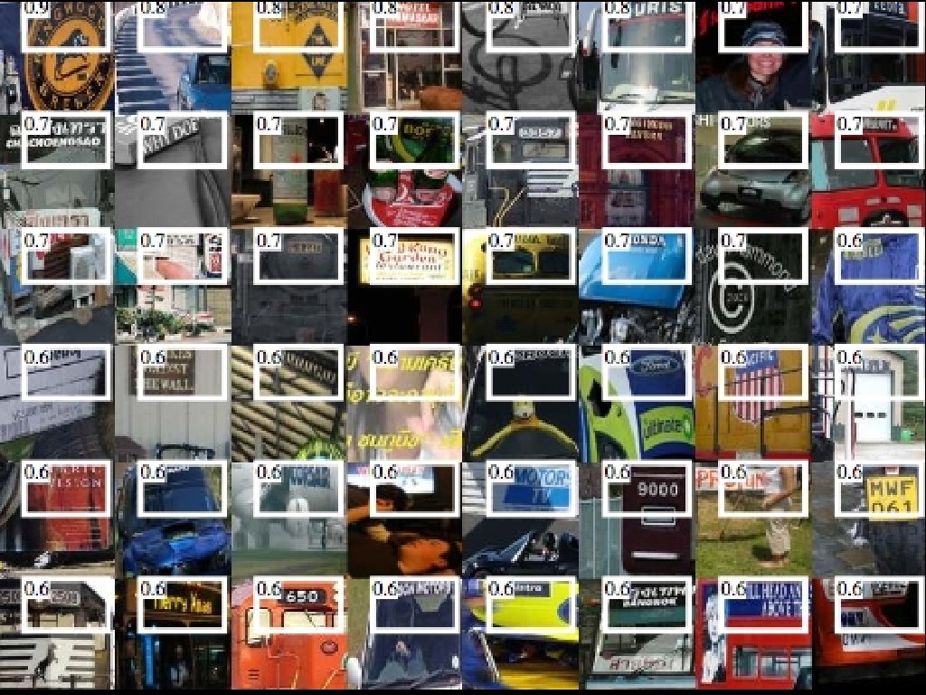
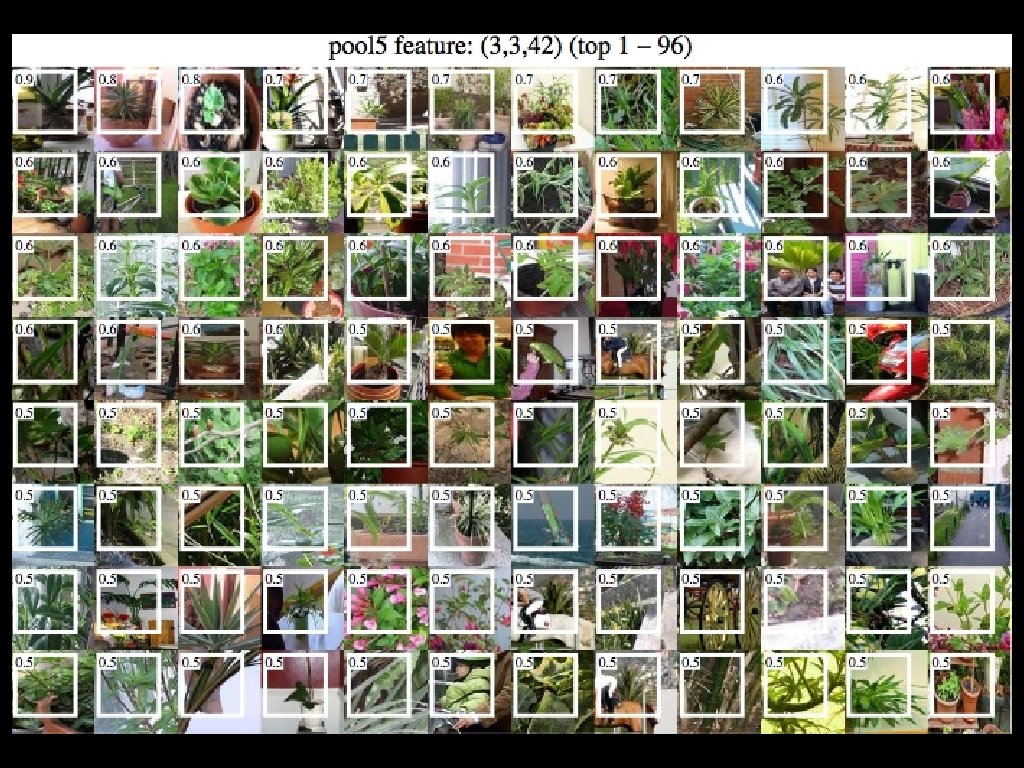
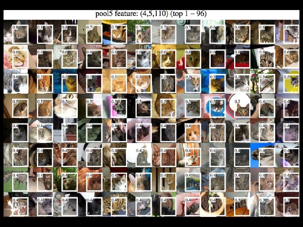
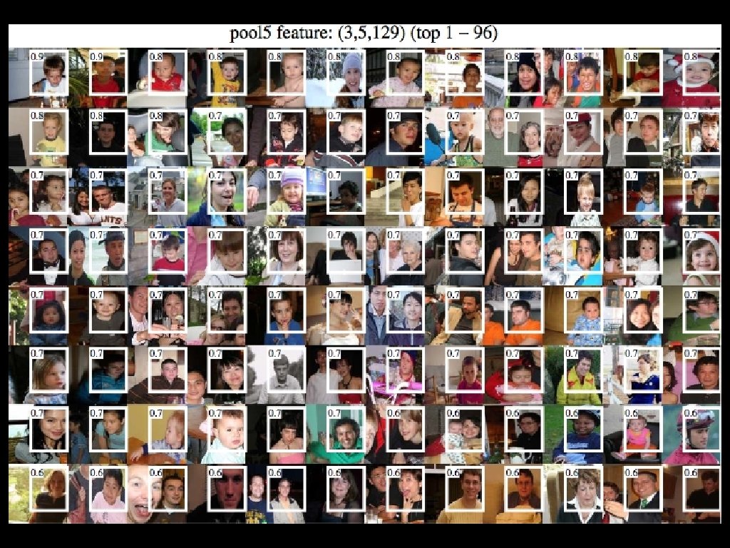
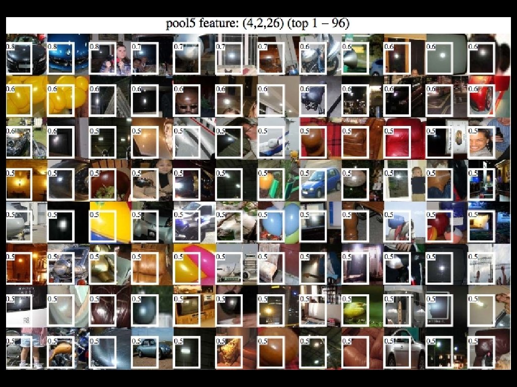
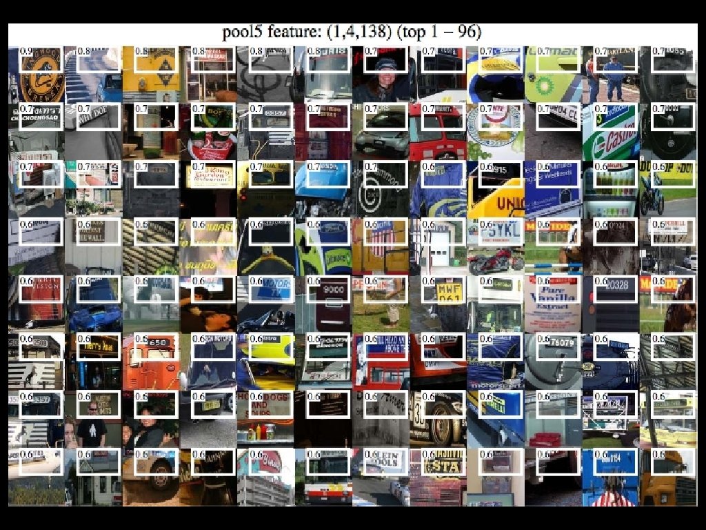
What did the network learn?

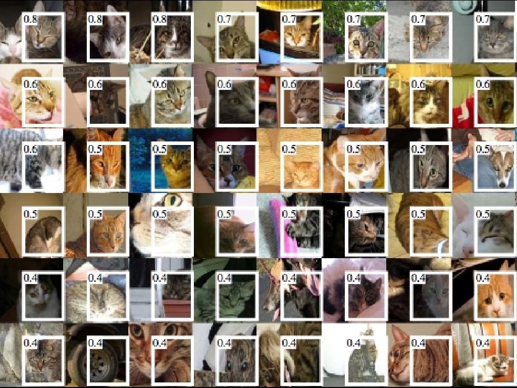
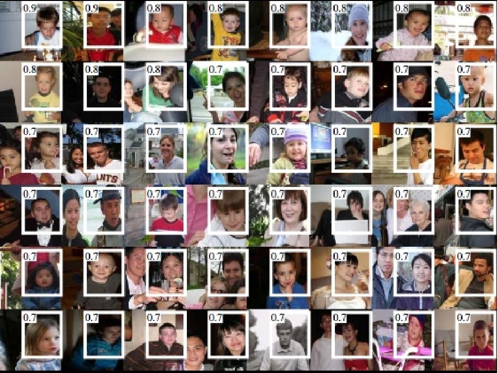
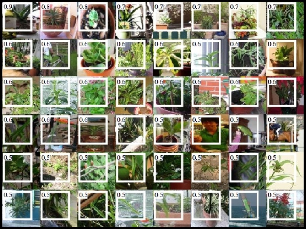
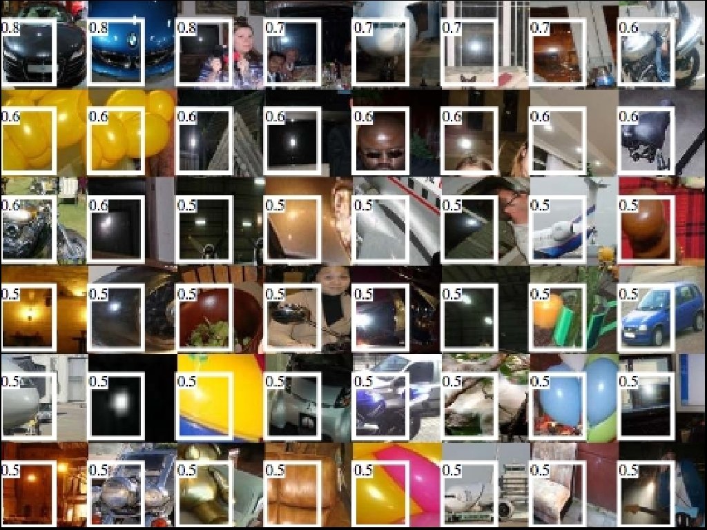
What did the network learn? “stimulus” ← feature channels → y x pool 5 feature map

What did the network learn? “stimulus” 227 pixels 6 cells ← feature channels → y x 6 y 227 x pool 5 feature map feature position receptive field Visualize images that activate pool 5 a feature

Take away - Dramatically better PASCAL m. AP - R-CNN outperforms other CNN-based methods on Image. Net detection - Detection speed is manageable (~11 s / image) - Scales very well with number of categories (30 ms for 20 → 200 classes!) - R-CNN is simple and completely open source

Semantic segmentation CPMC segments (Carreira & Sminchisescu) full fg

Semantic segmentation CPMC segments (Carreira & Sminchisescu) full fg VOC 2011 test Bonn second-order pooling (Carreira et al. ) 47. 6% R-CNN fc 6 full+fg (no fine-tuning) 47. 9% Improved to 50. 5% in our upcoming ECCV’ 14 work: Simultaneous Localization and Detection. Hariharan et al.

Get the code and models! bit. ly/rcnn-cvpr 14

Supplementary slides follow

Pre-trained CNN + SVMs (no FT) Regionlets (Wang et al. 2013) VOC 2007 VOC 2010 41. 7% 39. 7% Seg. DPM (Fidler et al. 2013) 40. 4% R-CNN pool 5 44. 2% R-CNN fc 6 46. 2% R-CNN fc 7 44. 7% R-CNN FT pool 5 47. 5% R-CNN FT fc 6 53. 2% R-CNN FT fc 7 54. 1% 50. 2% metric: mean average precision (higher is better)

False positive analysis No fine-tuning Analysis software: D. Hoiem, Y. Chodpathumwan, and Q. Dai. “Diagnosing Error in Object Detectors. ” ECCV, 2012.

False positive analysis After fine-tuning

False positive analysis After boundingbox regression

What did the network learn? z y y x x pool 5 “data cube” unit position Visualize pool 5 units receptive field

Comparison with DPM R-CNN DPM v 5 animals

Localization errors dominate background animals dissimilar classes vehicles localization furniture Analysis software: D. Hoiem, Y. Chodpathumwan, and Q. Dai. Diagnosing Error in Object Detectors. ECCV, 2012.