MN 50324 MAF Corporate Finance Semester 2 20089

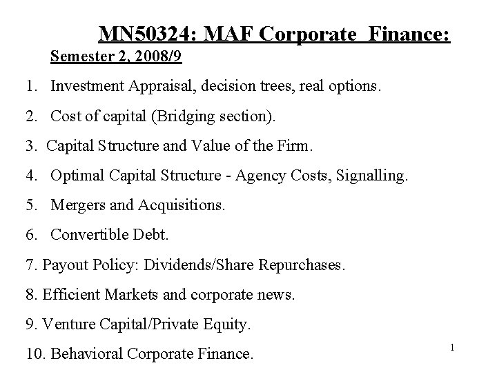
MN 50324: MAF Corporate Finance: Semester 2, 2008/9 1. Investment Appraisal, decision trees, real options. 2. Cost of capital (Bridging section). 3. Capital Structure and Value of the Firm. 4. Optimal Capital Structure - Agency Costs, Signalling. 5. Mergers and Acquisitions. 6. Convertible Debt. 7. Payout Policy: Dividends/Share Repurchases. 8. Efficient Markets and corporate news. 9. Venture Capital/Private Equity. 10. Behavioral Corporate Finance. 1

“Skills” required for the course • Numerical/analytical. • Conceptual ability (Essays). • Game Theory. 2

Assessment • 100% Exam: • - essay section. • - Analytical Section (numerical/game theoretic). • There are seminars (practice/feedback). • There will be revision sessions: with analytical/ essay practice! 3

Game-Theory • Game-theory has been used extensively in analysing corporate finance decisions. • Particularly, game theory is used to analyse strategic interaction between ‘players’: eg competing firms (in real option to delay); eg: interactions between managers and investors (in capital structure), venture capitalists and managers. • Games of asymmetric information: signalling games (debt/dividends etc) 4

Life-cycle of a Firm • Start-up Finance (venture capital) • IPOs. • Financial decision-making of existing publically-listed firms (investment appraisal/capital structure/dividend policy). • M and A/ private Equity. 5

Rational/behavioural debate • • Efficient markets hypothesis/ rational agents. Behavioural Corporate Finance => Irrational/biased managers. Irrational/biased investors. 6

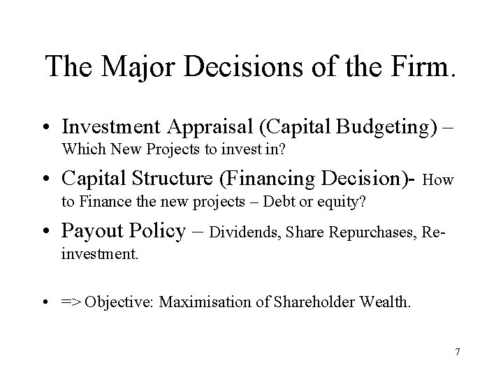
The Major Decisions of the Firm. • Investment Appraisal (Capital Budgeting) – Which New Projects to invest in? • Capital Structure (Financing Decision)- How to Finance the new projects – Debt or equity? • Payout Policy – Dividends, Share Repurchases, Reinvestment. • => Objective: Maximisation of Shareholder Wealth. 7

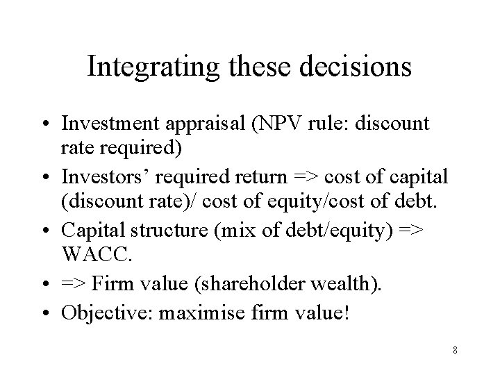
Integrating these decisions • Investment appraisal (NPV rule: discount rate required) • Investors’ required return => cost of capital (discount rate)/ cost of equity/cost of debt. • Capital structure (mix of debt/equity) => WACC. • => Firm value (shareholder wealth). • Objective: maximise firm value! 8

1. Investment Appraisal. • Objective: Take projects that increase shareholder wealth (Value-adding projects). • Investment Appraisal Techniques: NPV, IRR, Payback, ARR, Real Options…. • Which one is the Best rule for shareholder wealth maximisation? 9

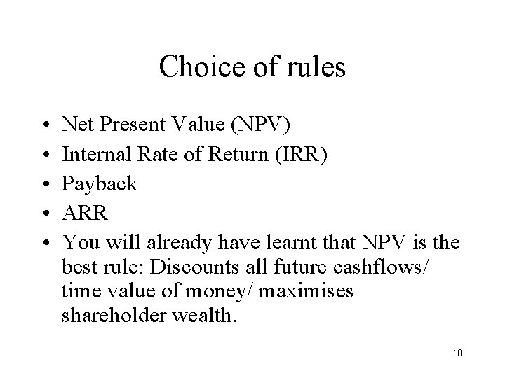
Choice of rules • • • Net Present Value (NPV) Internal Rate of Return (IRR) Payback ARR You will already have learnt that NPV is the best rule: Discounts all future cashflows/ time value of money/ maximises shareholder wealth. 10

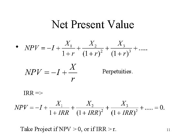
Net Present Value • Perpetuities. IRR => Take Project if NPV > 0, or if IRR > r. 11

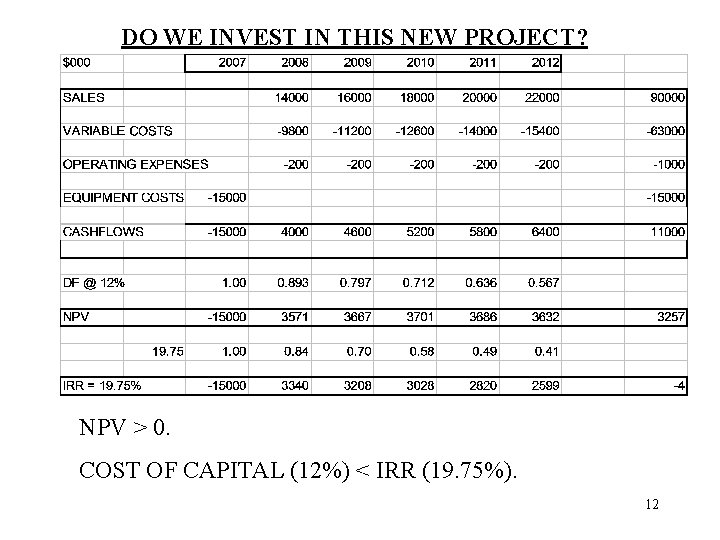
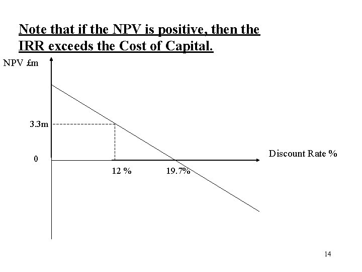
DO WE INVEST IN THIS NEW PROJECT? NPV > 0. COST OF CAPITAL (12%) < IRR (19. 75%). 12

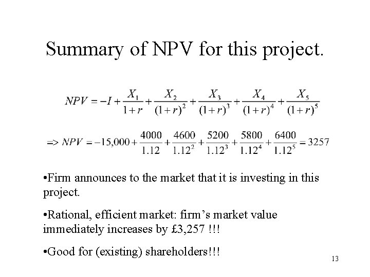
Summary of NPV for this project. • Firm announces to the market that it is investing in this project. • Rational, efficient market: firm’s market value immediately increases by £ 3, 257 !!! • Good for (existing) shareholders!!! 13

Note that if the NPV is positive, then the IRR exceeds the Cost of Capital. NPV £m 3. 3 m Discount Rate % 0 12 % 19. 7% 14

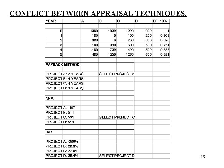
CONFLICT BETWEEN APPRAISAL TECHNIQUES. 15

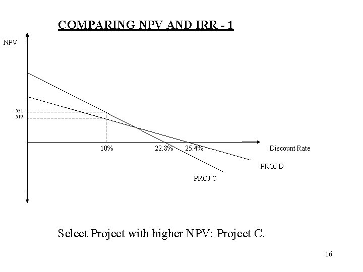
COMPARING NPV AND IRR - 1 NPV 531 519 10% 22. 8% 25. 4% Discount Rate PROJ D PROJ C Select Project with higher NPV: Project C. 16

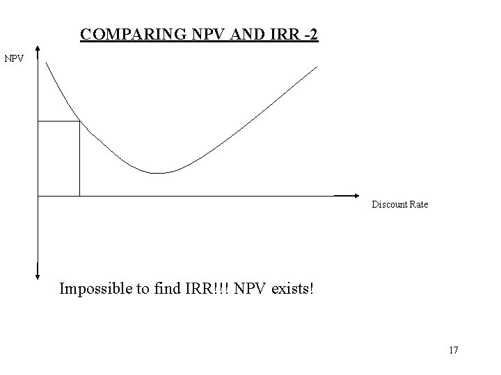
COMPARING NPV AND IRR -2 NPV Discount Rate Impossible to find IRR!!! NPV exists! 17

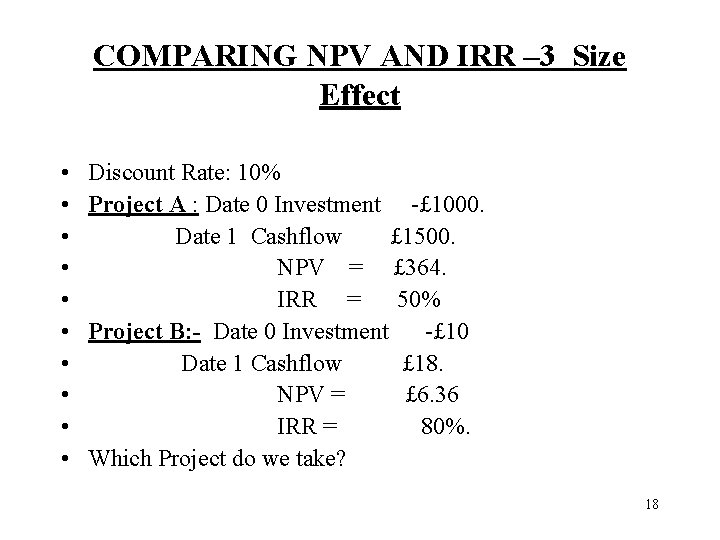
COMPARING NPV AND IRR – 3 Size Effect • • • Discount Rate: 10% Project A : Date 0 Investment -£ 1000. Date 1 Cashflow £ 1500. NPV = £ 364. IRR = 50% Project B: - Date 0 Investment -£ 10 Date 1 Cashflow £ 18. NPV = £ 6. 36 IRR = 80%. Which Project do we take? 18

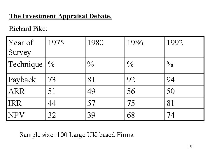
The Investment Appraisal Debate. Richard Pike: Year of 1975 Survey Technique % 1980 1986 1992 % % % Payback ARR IRR NPV 81 49 57 39 92 56 75 68 94 50 81 74 73 51 44 32 Sample size: 100 Large UK based Firms. 19

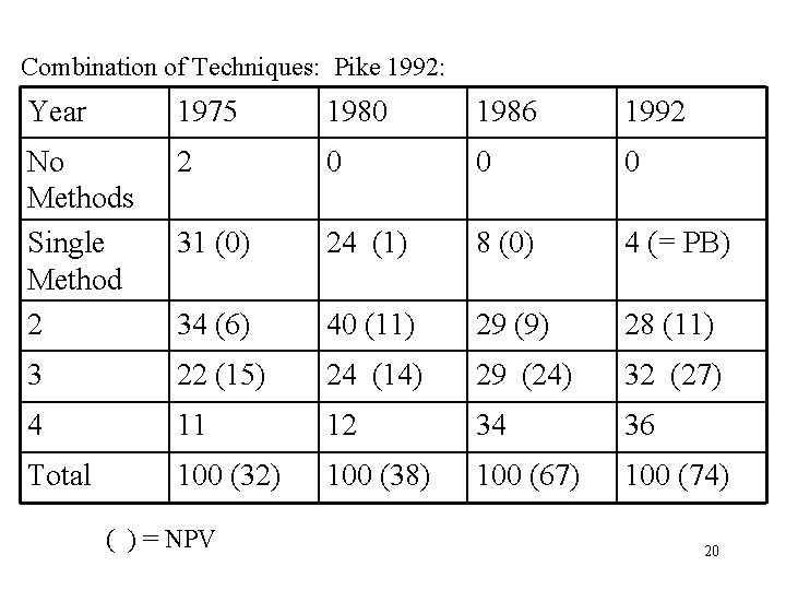
Combination of Techniques: Pike 1992: Year 1975 1980 1986 1992 No Methods Single Method 2 2 0 0 0 31 (0) 24 (1) 8 (0) 4 (= PB) 34 (6) 40 (11) 29 (9) 28 (11) 3 22 (15) 24 (14) 29 (24) 32 (27) 4 11 12 34 36 Total 100 (32) 100 (38) 100 (67) 100 (74) ( ) = NPV 20

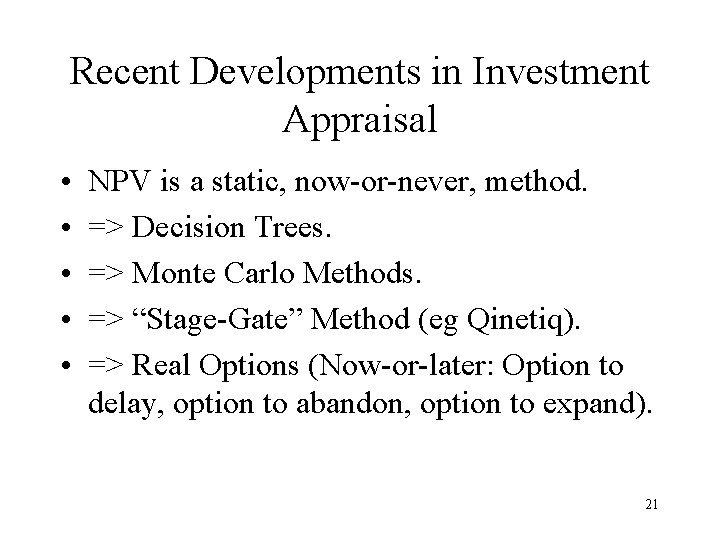
Recent Developments in Investment Appraisal • • • NPV is a static, now-or-never, method. => Decision Trees. => Monte Carlo Methods. => “Stage-Gate” Method (eg Qinetiq). => Real Options (Now-or-later: Option to delay, option to abandon, option to expand). 21

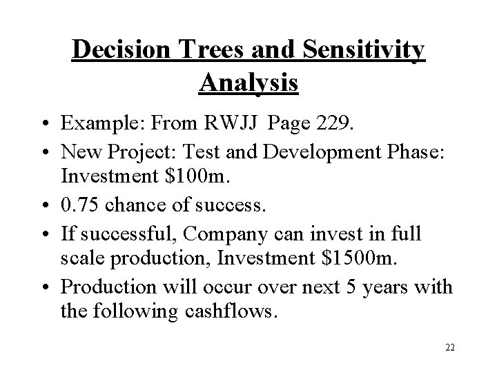
Decision Trees and Sensitivity Analysis • Example: From RWJJ Page 229. • New Project: Test and Development Phase: Investment $100 m. • 0. 75 chance of success. • If successful, Company can invest in full scale production, Investment $1500 m. • Production will occur over next 5 years with the following cashflows. 22

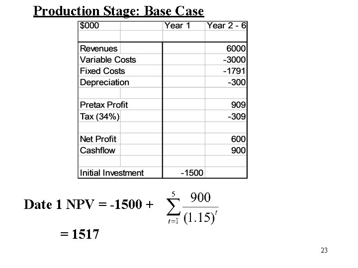
Production Stage: Base Case Date 1 NPV = -1500 + = 1517 23

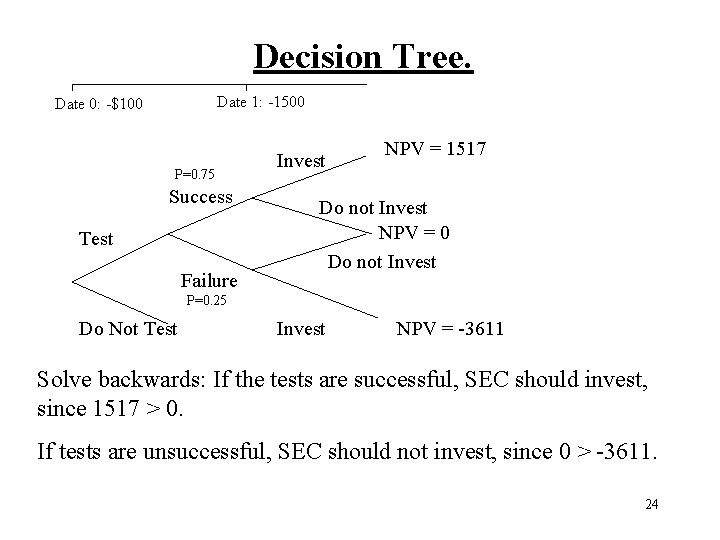
Decision Tree. Date 1: -1500 Date 0: -$100 P=0. 75 Success Test Failure Invest NPV = 1517 Do not Invest NPV = 0 Do not Invest P=0. 25 Do Not Test Invest NPV = -3611 Solve backwards: If the tests are successful, SEC should invest, since 1517 > 0. If tests are unsuccessful, SEC should not invest, since 0 > -3611. 24

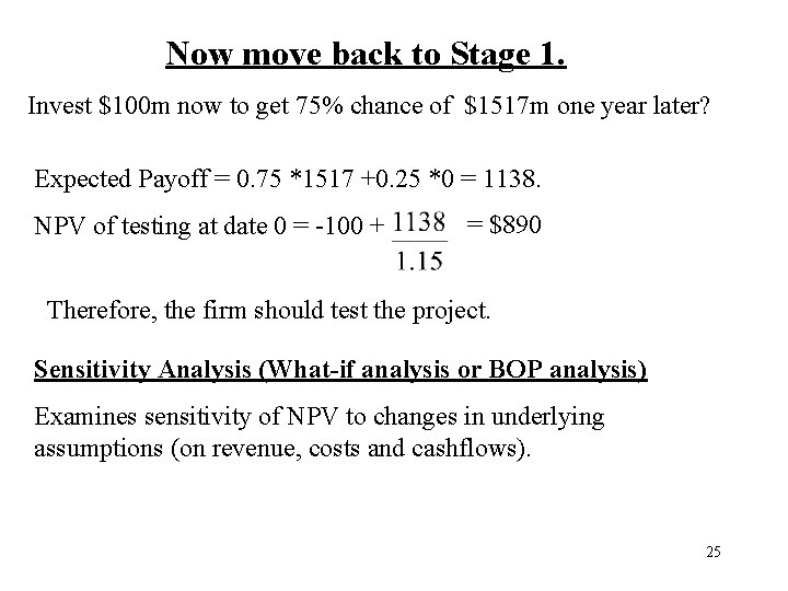
Now move back to Stage 1. Invest $100 m now to get 75% chance of $1517 m one year later? Expected Payoff = 0. 75 *1517 +0. 25 *0 = 1138. NPV of testing at date 0 = -100 + = $890 Therefore, the firm should test the project. Sensitivity Analysis (What-if analysis or BOP analysis) Examines sensitivity of NPV to changes in underlying assumptions (on revenue, costs and cashflows). 25

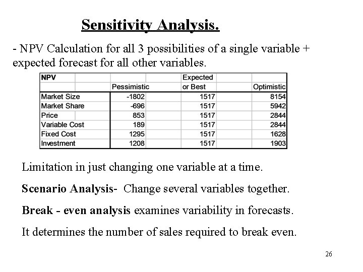
Sensitivity Analysis. - NPV Calculation for all 3 possibilities of a single variable + expected forecast for all other variables. Limitation in just changing one variable at a time. Scenario Analysis- Change several variables together. Break - even analysis examines variability in forecasts. It determines the number of sales required to break even. 26

Monte Carlo Method (RWJJ pp 237241. • Monte-Carlo simulation: further attempt to model real-world uncertainty. • Monte-Carlo? Analysing project uncertainty same way that you would analyse gambling strategies. 27

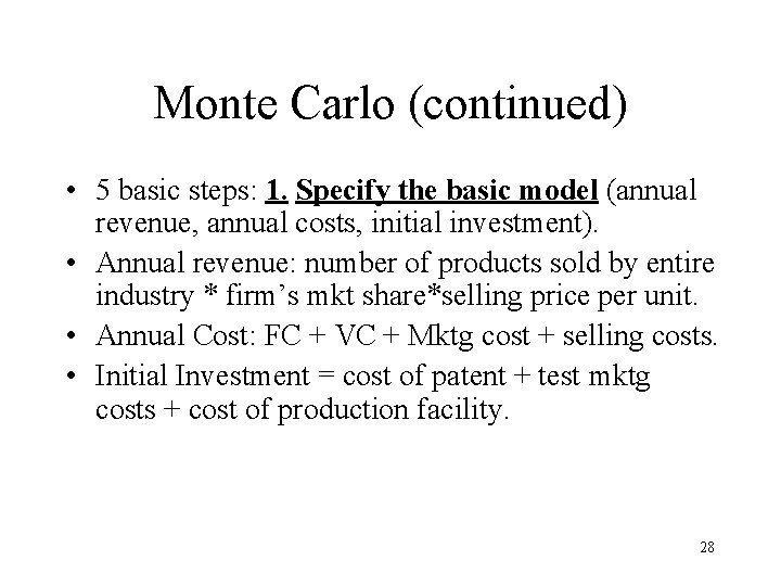
Monte Carlo (continued) • 5 basic steps: 1. Specify the basic model (annual revenue, annual costs, initial investment). • Annual revenue: number of products sold by entire industry * firm’s mkt share*selling price per unit. • Annual Cost: FC + VC + Mktg cost + selling costs. • Initial Investment = cost of patent + test mktg costs + cost of production facility. 28

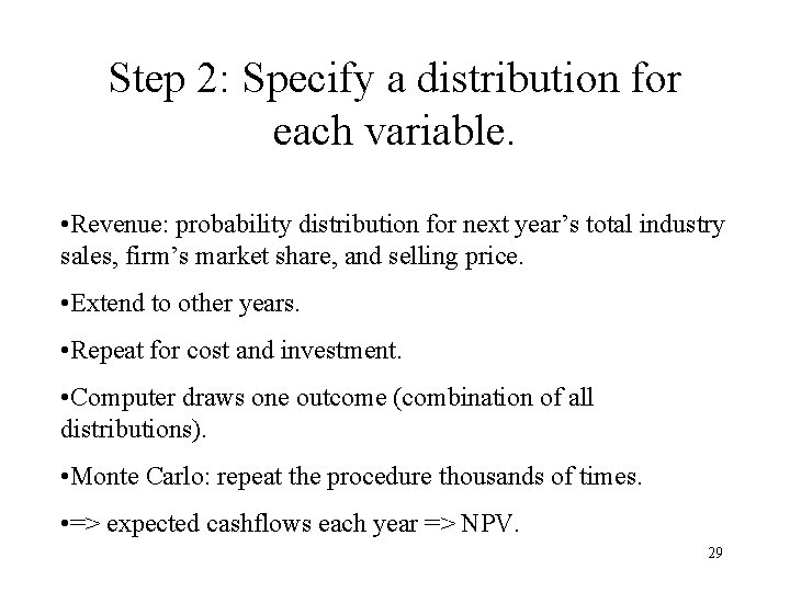
Step 2: Specify a distribution for each variable. • Revenue: probability distribution for next year’s total industry sales, firm’s market share, and selling price. • Extend to other years. • Repeat for cost and investment. • Computer draws one outcome (combination of all distributions). • Monte Carlo: repeat the procedure thousands of times. • => expected cashflows each year => NPV. 29

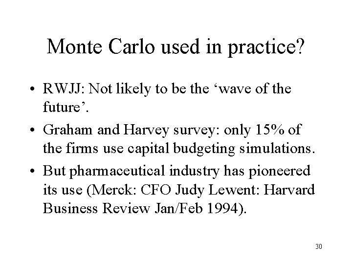
Monte Carlo used in practice? • RWJJ: Not likely to be the ‘wave of the future’. • Graham and Harvey survey: only 15% of the firms use capital budgeting simulations. • But pharmaceutical industry has pioneered its use (Merck: CFO Judy Lewent: Harvard Business Review Jan/Feb 1994). 30

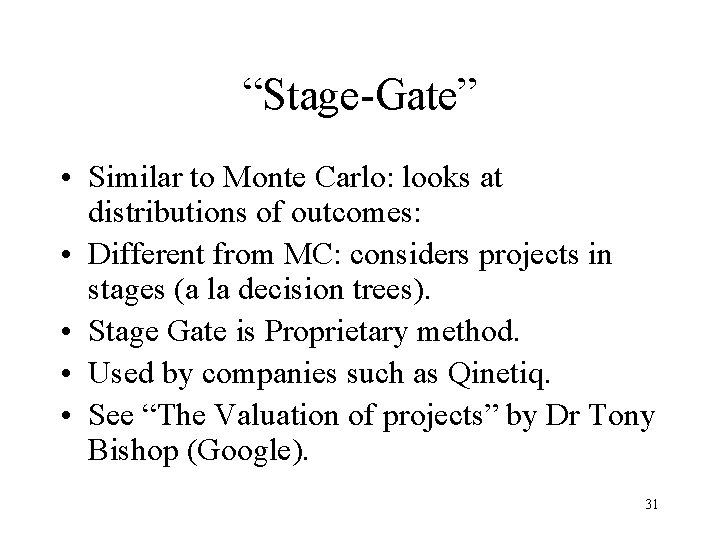
“Stage-Gate” • Similar to Monte Carlo: looks at distributions of outcomes: • Different from MC: considers projects in stages (a la decision trees). • Stage Gate is Proprietary method. • Used by companies such as Qinetiq. • See “The Valuation of projects” by Dr Tony Bishop (Google). 31

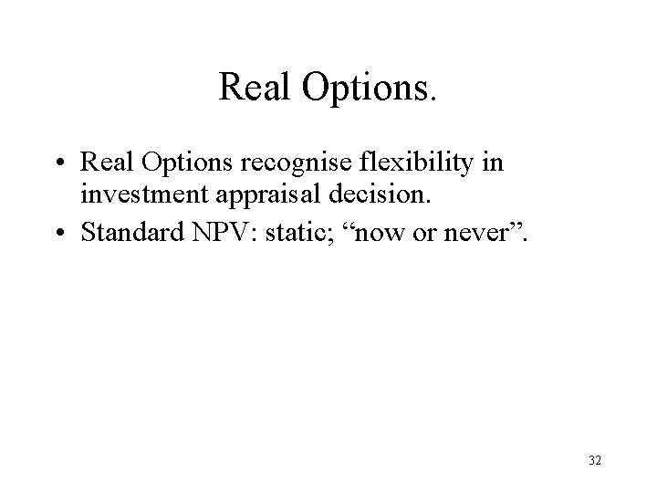
Real Options. • Real Options recognise flexibility in investment appraisal decision. • Standard NPV: static; “now or never”. 32

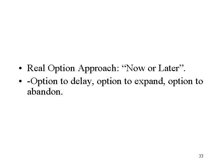
• Real Option Approach: “Now or Later”. • -Option to delay, option to expand, option to abandon. 33

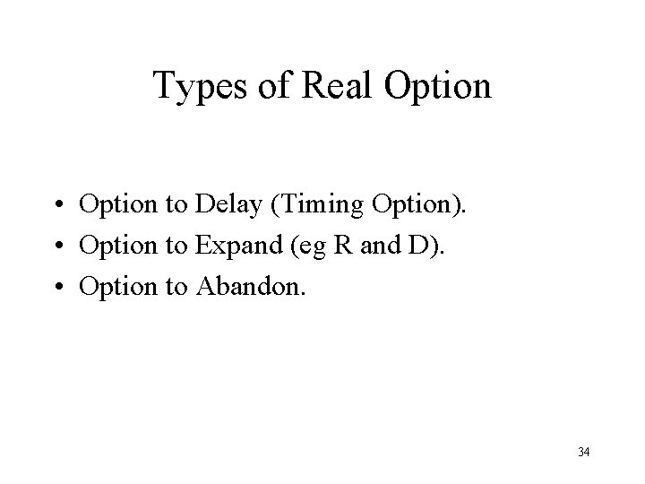
Types of Real Option • Option to Delay (Timing Option). • Option to Expand (eg R and D). • Option to Abandon. 34

Valuation of Real Options • Binomial Pricing Model • Black-Scholes formula 35

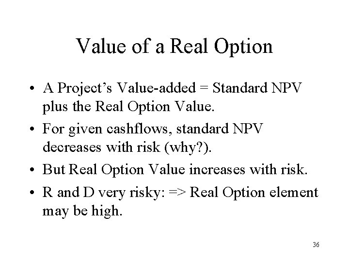
Value of a Real Option • A Project’s Value-added = Standard NPV plus the Real Option Value. • For given cashflows, standard NPV decreases with risk (why? ). • But Real Option Value increases with risk. • R and D very risky: => Real Option element may be high. 36

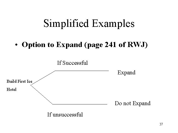
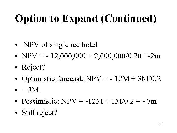
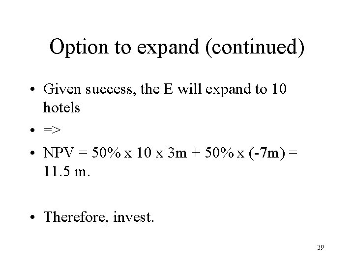
Simplified Examples • Option to Expand (page 241 of RWJ) If Successful Expand Build First Ice Hotel Do not Expand If unsuccessful 37

Option to Expand (Continued) • • NPV of single ice hotel NPV = - 12, 000 + 2, 000/0. 20 =-2 m Reject? Optimistic forecast: NPV = - 12 M + 3 M/0. 2 = 3 M. Pessimistic: NPV = -12 M + 1 M/0. 2 = - 7 m Still reject? 38

Option to expand (continued) • Given success, the E will expand to 10 hotels • => • NPV = 50% x 10 x 3 m + 50% x (-7 m) = 11. 5 m. • Therefore, invest. 39

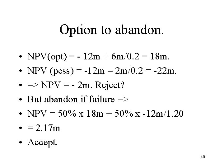
Option to abandon. • • NPV(opt) = - 12 m + 6 m/0. 2 = 18 m. NPV (pess) = -12 m – 2 m/0. 2 = -22 m. => NPV = - 2 m. Reject? But abandon if failure => NPV = 50% x 18 m + 50% x -12 m/1. 20 = 2. 17 m Accept. 40

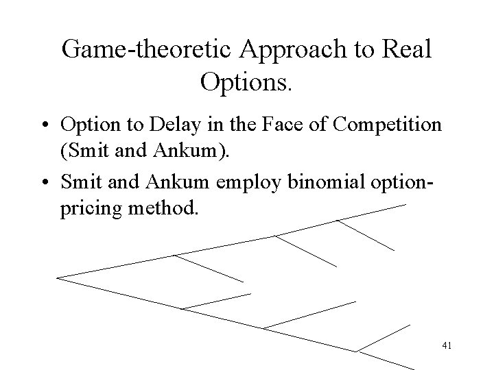
Game-theoretic Approach to Real Options. • Option to Delay in the Face of Competition (Smit and Ankum). • Smit and Ankum employ binomial optionpricing method. 41

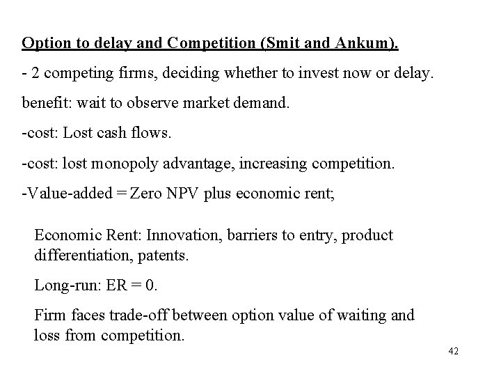
Option to delay and Competition (Smit and Ankum). - 2 competing firms, deciding whether to invest now or delay. benefit: wait to observe market demand. -cost: Lost cash flows. -cost: lost monopoly advantage, increasing competition. -Value-added = Zero NPV plus economic rent; Economic Rent: Innovation, barriers to entry, product differentiation, patents. Long-run: ER = 0. Firm faces trade-off between option value of waiting and loss from competition. 42

Other Papers analysing game theoretic approach to Real Options • Smit and Trigeorgis (RFE 2006). • Imai and Watanabe (Google 2004) • => Class exercise. 43

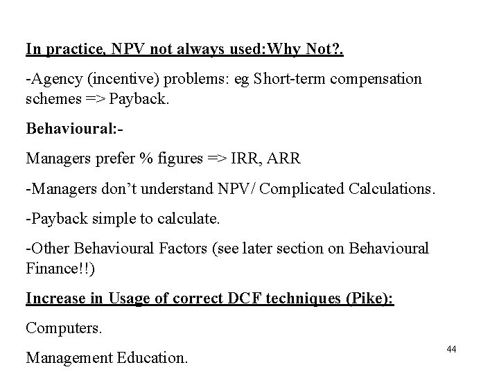
In practice, NPV not always used: Why Not? . -Agency (incentive) problems: eg Short-term compensation schemes => Payback. Behavioural: Managers prefer % figures => IRR, ARR -Managers don’t understand NPV/ Complicated Calculations. -Payback simple to calculate. -Other Behavioural Factors (see later section on Behavioural Finance!!) Increase in Usage of correct DCF techniques (Pike): Computers. Management Education. 44

Game-theoretic model of NPV. • Israel and Berkovitch RFS 2004. • NPV is seen as standard value-maximising technique. • But IB’s game-theoretic approach considers the impact of agency and assymetric information problems 45

Israel and Berkovitch (continued) • • A firm consisting of two components: 1: Top management (Headquarters) 2. divisional managers (“the manager”). Objective of headquarters: Maximisation of shareholder value. • Objective of manager: maximise her own utility. 46

Israel and Berkovitch (continued) • HQ needs to design a monitoring and incentive mechanism to deal with these conflicting objectives. • => capital allocation system specifying: • A capital budgeting rule (eg NPV/IRR) and a wage compensation for divisional managers. 47

Israel and Berkovitch • Paper demonstrates the ingredients of a game-theoretic approach. • Players. • Objectives (utility functions to maximise) • Strategies. • Payoffs. 48

2. Cost of Capital/discount rate/investors’ required return. • What discount rate to use in NPV/ valuation? • Portfolio analysis => Investors’ required return as a compensation for risk • => CAPM (capital asset pricing model) => cost of equity (risk-averse equity-holders’ required return): increases with risk. 49

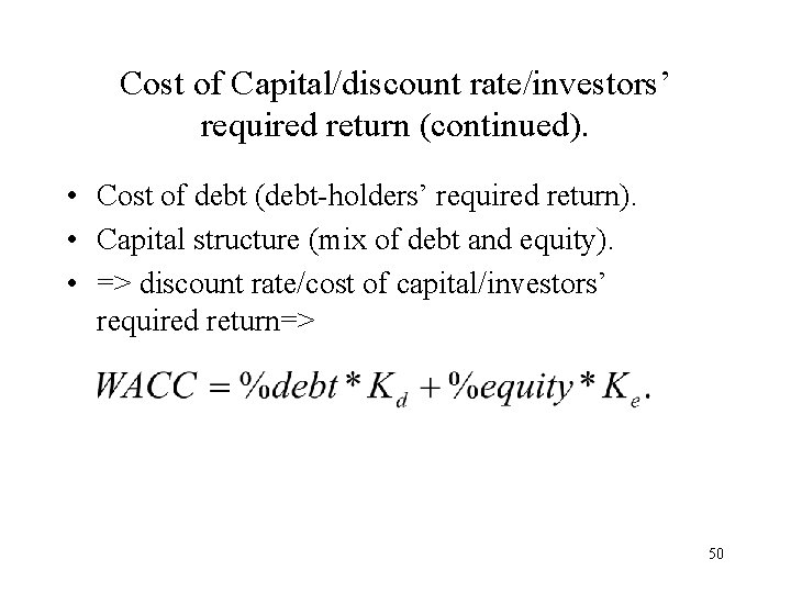
Cost of Capital/discount rate/investors’ required return (continued). • Cost of debt (debt-holders’ required return). • Capital structure (mix of debt and equity). • => discount rate/cost of capital/investors’ required return=> 50

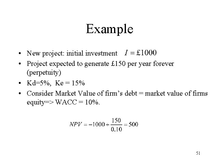
Example • New project: initial investment • Project expected to generate £ 150 per year forever (perpetuity) • Kd=5%, Ke = 15% • Consider Market Value of firm’s debt = market value of firms equity=> WACC = 10%. 51

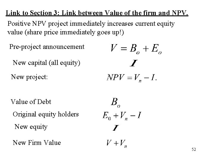
Link to Section 3: Link between Value of the firm and NPV. Positive NPV project immediately increases current equity value (share price immediately goes up!) Pre-project announcement New capital (all equity) New project: Value of Debt Original equity holders New equity New Firm Value 52

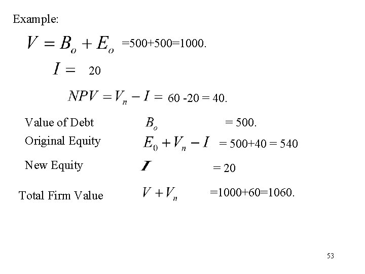
Example: =500+500=1000. 20 60 -20 = 40. Value of Debt Original Equity New Equity Total Firm Value = 500+40 = 540 = 20 =1000+60=1060. 53

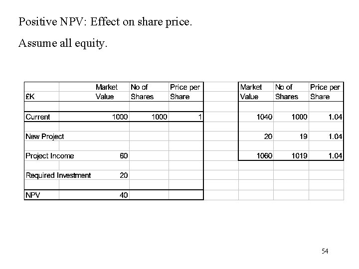
Positive NPV: Effect on share price. Assume all equity. 54

• For now, we assume rationality of agents, and efficient markets (=> markets react immediately to news)! • Analyse efficient markets in section 6 • And behavioural corporate finance in section 9. 55

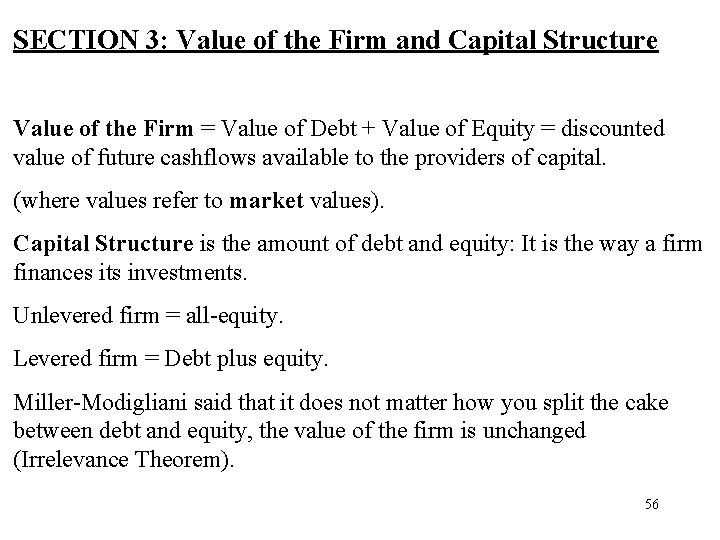
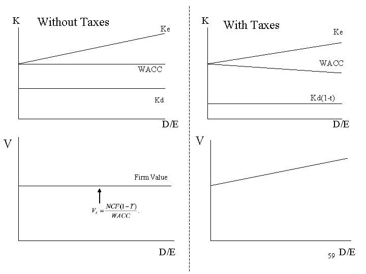
SECTION 3: Value of the Firm and Capital Structure Value of the Firm = Value of Debt + Value of Equity = discounted value of future cashflows available to the providers of capital. (where values refer to market values). Capital Structure is the amount of debt and equity: It is the way a firm finances its investments. Unlevered firm = all-equity. Levered firm = Debt plus equity. Miller-Modigliani said that it does not matter how you split the cake between debt and equity, the value of the firm is unchanged (Irrelevance Theorem). 56

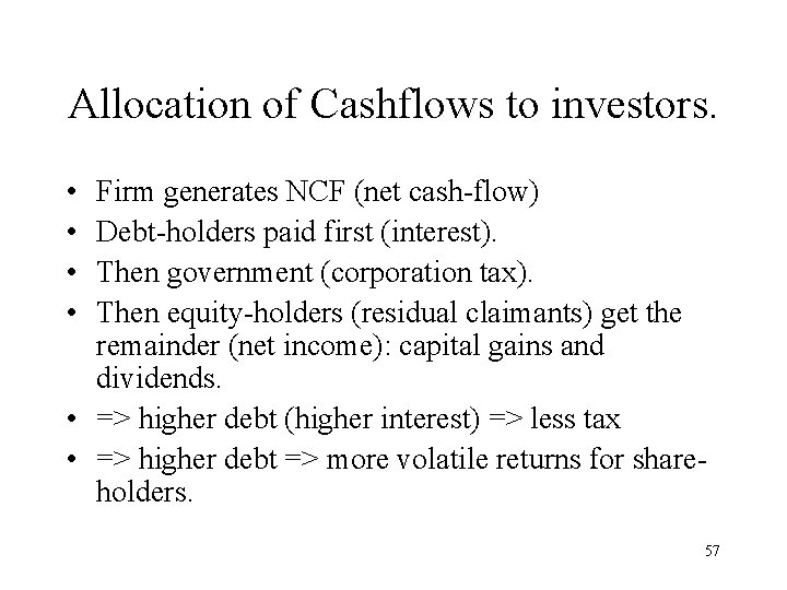
Allocation of Cashflows to investors. • • Firm generates NCF (net cash-flow) Debt-holders paid first (interest). Then government (corporation tax). Then equity-holders (residual claimants) get the remainder (net income): capital gains and dividends. • => higher debt (higher interest) => less tax • => higher debt => more volatile returns for shareholders. 57

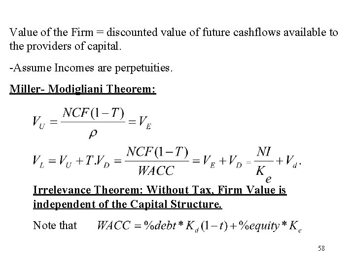
Value of the Firm = discounted value of future cashflows available to the providers of capital. -Assume Incomes are perpetuities. Miller- Modigliani Theorem: Irrelevance Theorem: Without Tax, Firm Value is independent of the Capital Structure. Note that 58

K Without Taxes Ke K With Taxes Ke WACC Kd(1 -t) Kd D/E V V Firm Value D/E 59 D/E

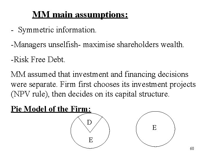
MM main assumptions: - Symmetric information. -Managers unselfish- maximise shareholders wealth. -Risk Free Debt. MM assumed that investment and financing decisions were separate. Firm first chooses its investment projects (NPV rule), then decides on its capital structure. Pie Model of the Firm: D E E 60

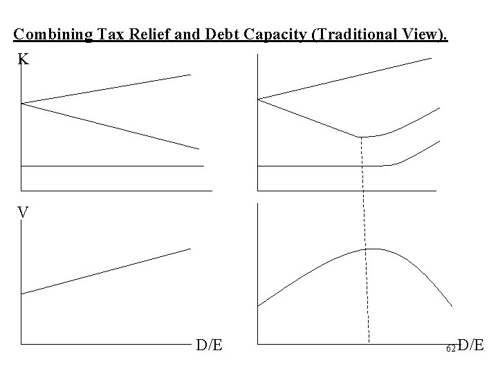
MM irrelevance theorem- firm can use any mix of debt and equity – this is unsatisfactory as a policy tool. Searching for the Optimal Capital Structure. -Tax benefits of debt. -Asymmetric information- Signalling. -Agency Costs (selfish managers). -Debt Capacity and Risky Debt. Optimal Capital Structure maximises firm value. 61

Combining Tax Relief and Debt Capacity (Traditional View). K V D/E 62 D/E

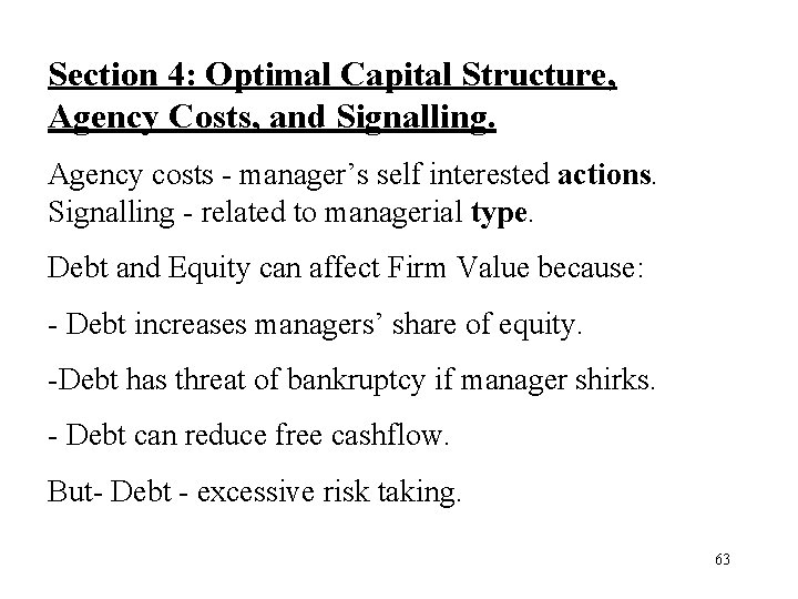
Section 4: Optimal Capital Structure, Agency Costs, and Signalling. Agency costs - manager’s self interested actions. Signalling - related to managerial type. Debt and Equity can affect Firm Value because: - Debt increases managers’ share of equity. -Debt has threat of bankruptcy if manager shirks. - Debt can reduce free cashflow. But- Debt - excessive risk taking. 63

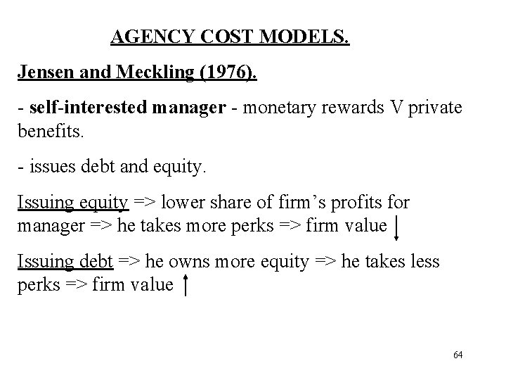
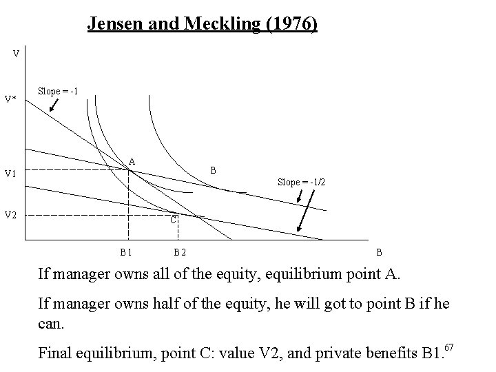
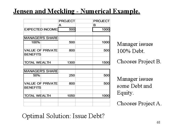
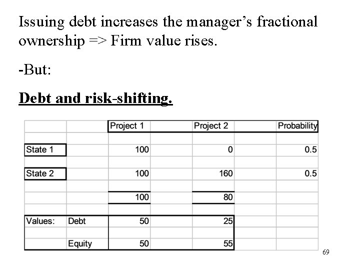
AGENCY COST MODELS. Jensen and Meckling (1976). - self-interested manager - monetary rewards V private benefits. - issues debt and equity. Issuing equity => lower share of firm’s profits for manager => he takes more perks => firm value Issuing debt => he owns more equity => he takes less perks => firm value 64

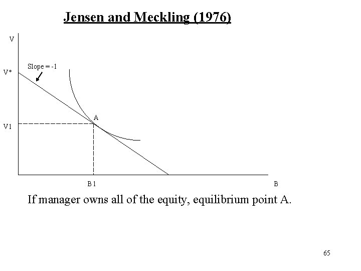
Jensen and Meckling (1976) V V* Slope = -1 A V 1 B If manager owns all of the equity, equilibrium point A. 65

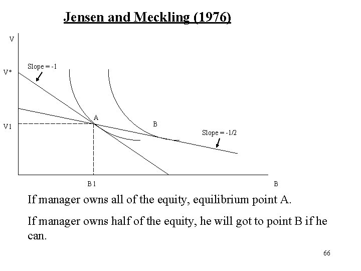
Jensen and Meckling (1976) V V* Slope = -1 A V 1 B Slope = -1/2 B 1 B If manager owns all of the equity, equilibrium point A. If manager owns half of the equity, he will got to point B if he can. 66

Jensen and Meckling (1976) V V* Slope = -1 A B V 1 Slope = -1/2 V 2 C B 1 B 2 B If manager owns all of the equity, equilibrium point A. If manager owns half of the equity, he will got to point B if he can. Final equilibrium, point C: value V 2, and private benefits B 1. 67

Jensen and Meckling - Numerical Example. Manager issues 100% Debt. Chooses Project B. Manager issues some Debt and Equity. Chooses Project A. Optimal Solution: Issue Debt? 68

Issuing debt increases the manager’s fractional ownership => Firm value rises. -But: Debt and risk-shifting. 69

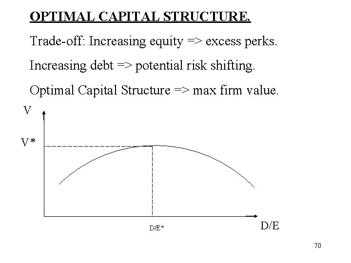
OPTIMAL CAPITAL STRUCTURE. Trade-off: Increasing equity => excess perks. Increasing debt => potential risk shifting. Optimal Capital Structure => max firm value. V V* D/E 70

Other Agency Cost Reasons for Optimal Capital structure. Debt - bankruptcy threat - manager increases effort level. (eg Hart, Dewatripont and Tirole). Debt reduces free cashflow problem (eg Jensen 1986). 71

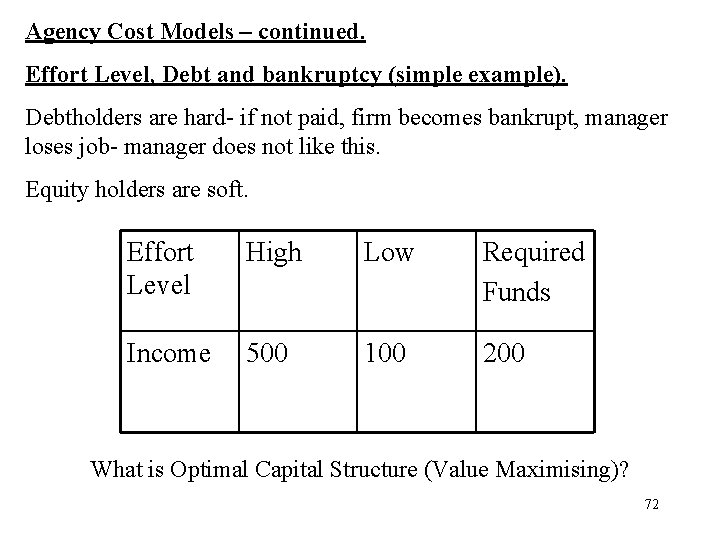
Agency Cost Models – continued. Effort Level, Debt and bankruptcy (simple example). Debtholders are hard- if not paid, firm becomes bankrupt, manager loses job- manager does not like this. Equity holders are soft. Effort Level High Low Required Funds Income 500 100 200 What is Optimal Capital Structure (Value Maximising)? 72

Firm needs to raise 200, using debt and equity. Manager only cares about keeping his job. He has a fixed income, not affected by firm value. a) If debt < 100, low effort. V = 100. Manager keeps job. b) If debt > 100: low effort, V < D => bankruptcy. Manager loses job. So, high effort level => V = 500 > D. No bankruptcy => Manager keeps job. High level of debt => high firm value. However: trade-off: may be costs of having high debt levels. 73

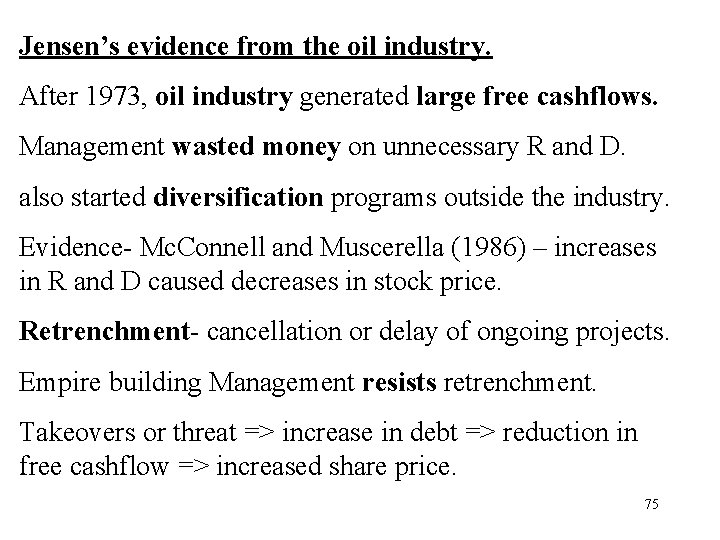
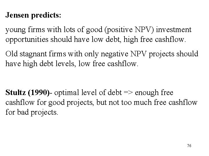
Free Cashflow Problem (Jensen 1986). -Managers have (negative NPV) pet projects. -Empire Building. => Firm Value reducing. Free Cashflow- Cashflow in excess of that required to fund all NPV projects. Jensen- benefit of debt in reducing free cashflow. 74

Jensen’s evidence from the oil industry. After 1973, oil industry generated large free cashflows. Management wasted money on unnecessary R and D. also started diversification programs outside the industry. Evidence- Mc. Connell and Muscerella (1986) – increases in R and D caused decreases in stock price. Retrenchment- cancellation or delay of ongoing projects. Empire building Management resists retrenchment. Takeovers or threat => increase in debt => reduction in free cashflow => increased share price. 75

Jensen predicts: young firms with lots of good (positive NPV) investment opportunities should have low debt, high free cashflow. Old stagnant firms with only negative NPV projects should have high debt levels, low free cashflow. Stultz (1990)- optimal level of debt => enough free cashflow for good projects, but not too much free cashflow for bad projects. 76

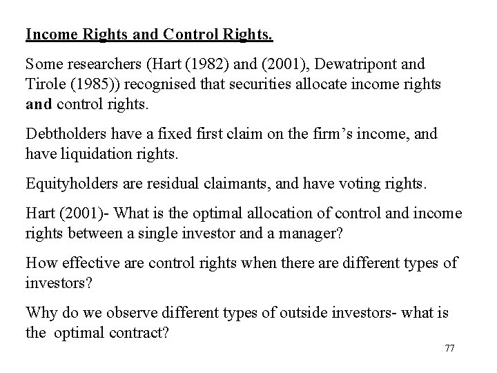
Income Rights and Control Rights. Some researchers (Hart (1982) and (2001), Dewatripont and Tirole (1985)) recognised that securities allocate income rights and control rights. Debtholders have a fixed first claim on the firm’s income, and have liquidation rights. Equityholders are residual claimants, and have voting rights. Hart (2001)- What is the optimal allocation of control and income rights between a single investor and a manager? How effective are control rights when there are different types of investors? Why do we observe different types of outside investors- what is the optimal contract? 77

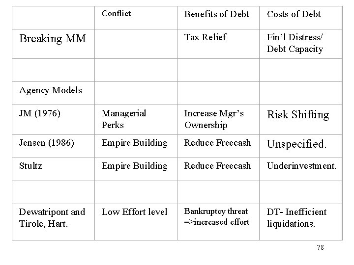
Conflict Breaking MM Benefits of Debt Costs of Debt Tax Relief Fin’l Distress/ Debt Capacity Agency Models JM (1976) Managerial Perks Increase Mgr’s Ownership Risk Shifting Jensen (1986) Empire Building Reduce Freecash Unspecified. Stultz Empire Building Reduce Freecash Underinvestment. Dewatripont and Tirole, Hart. Low Effort level Bankruptcy threat =>increased effort DT- Inefficient liquidations. 78

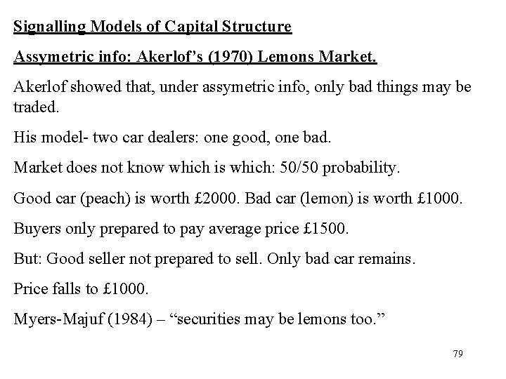
Signalling Models of Capital Structure Assymetric info: Akerlof’s (1970) Lemons Market. Akerlof showed that, under assymetric info, only bad things may be traded. His model- two car dealers: one good, one bad. Market does not know which is which: 50/50 probability. Good car (peach) is worth £ 2000. Bad car (lemon) is worth £ 1000. Buyers only prepared to pay average price £ 1500. But: Good seller not prepared to sell. Only bad car remains. Price falls to £ 1000. Myers-Majuf (1984) – “securities may be lemons too. ” 79

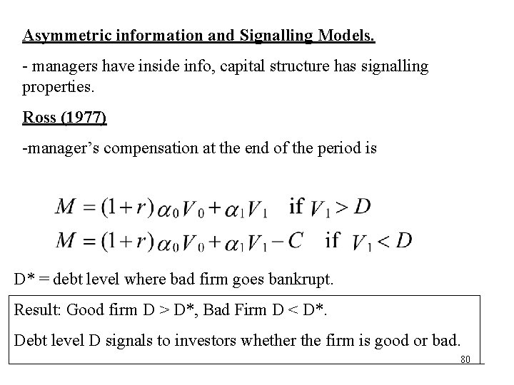
Asymmetric information and Signalling Models. - managers have inside info, capital structure has signalling properties. Ross (1977) -manager’s compensation at the end of the period is D* = debt level where bad firm goes bankrupt. Result: Good firm D > D*, Bad Firm D < D*. Debt level D signals to investors whether the firm is good or bad. 80

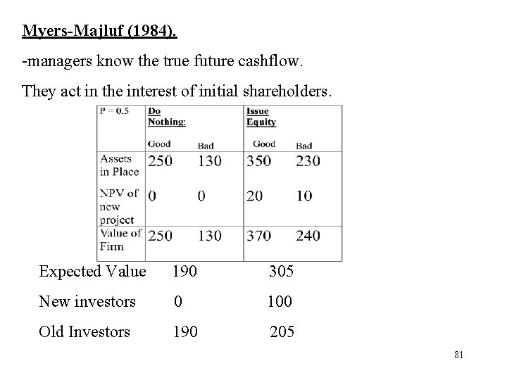
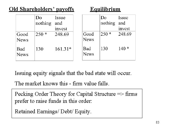
Myers-Majluf (1984). -managers know the true future cashflow. They act in the interest of initial shareholders. Expected Value 190 305 New investors 0 100 Old Investors 190 205 81

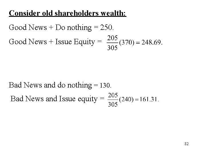
Consider old shareholders wealth: Good News + Do nothing = 250. Good News + Issue Equity = Bad News and do nothing = 130. Bad News and Issue equity = 82

Old Shareholders’ payoffs Equilibrium Issuing equity signals that the bad state will occur. The market knows this - firm value falls. Pecking Order Theory for Capital Structure => firms prefer to raise funds in this order: Retained Earnings/ Debt/ Equity. 83

Evidence on Capital structure and firm value. Debt Issued - Value Increases. Equity Issued- Value falls. However, difficult to analyse, as these capital structure changes may be accompanied by new investment. More promising - Exchange offers or swaps. Class discussion paper: Masulis (1980)- Highly significant Announcement effects: +7. 6% for leverage increasing exchange offers. -5. 4% for leverage decreasing exchange offers. 84

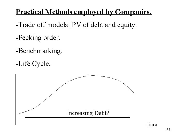
Practical Methods employed by Companies. -Trade off models: PV of debt and equity. -Pecking order. -Benchmarking. -Life Cycle. Increasing Debt? time 85

Trade-off Versus Pecking Order. • Empirical Tests. • Multiple Regression analysis (firm size/growth opportunities/tangibility of assets/profitability…. . • => Relationship between profitability and leverage (debt): positive => trade-off. • Or negative => Pecking order: • Why? 86

Capital Structure and Product Market Competition. • Research has recognised that firms’ financial decisions and product market decisions not made in isolation. • How does competition in the product market affect firms’ debt/equity decisions? • Limited liability models: Debt softens competition: higher comp => higher debt. • Predation models: higher competition leads to lower debt. (Why? ) 87

Game Theoretic Approach to Capital Structure. • Moral Hazard Model. • Asymmetric Information Model. • See BCF section 8 for incorporation of managerial overconfidence. 88

Cash-flow Rights and Control Rights • Debt-holders: first fixed claim on cashflows (cash-flow rights); liquidation rights in bas times (control rights)- hard investors. • Equity-holders: residual claimants on cashflows (cash-flow rights): voting rights in good times (control rights) – soft investors. • => minority shareholder rights versus blockholders. 89

Equity-holders’ control rights • • Voting rights. Soft: free-rider problems. Minority holders versus block-holders. Minority –holders versus insiders. Separation of ownership and control. Corporate Charter. Dual class of shares. Pyramids/tunelling etc. 90

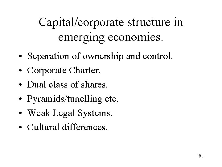
Capital/corporate structure in emerging economies. • • • Separation of ownership and control. Corporate Charter. Dual class of shares. Pyramids/tunelling etc. Weak Legal Systems. Cultural differences. 91

Game-theoretic approaches. • JFE special issue 1988 (Grossman and Hart, Stultz, Harris and Raviv). • Bebchuk (lecture slides to follow). • Garro Paulin and Fairchild (2006) Lecture slides to follow. 92

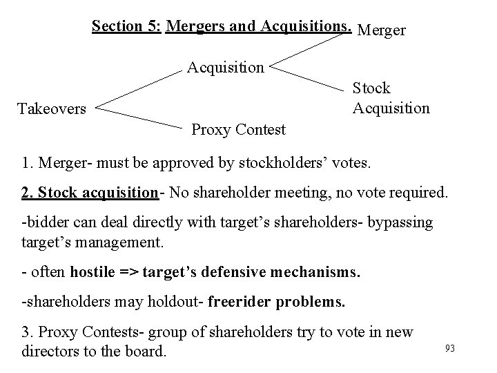
Section 5: Mergers and Acquisitions. Merger Acquisition Stock Acquisition Takeovers Proxy Contest 1. Merger- must be approved by stockholders’ votes. 2. Stock acquisition- No shareholder meeting, no vote required. -bidder can deal directly with target’s shareholders- bypassing target’s management. - often hostile => target’s defensive mechanisms. -shareholders may holdout- freerider problems. 3. Proxy Contests- group of shareholders try to vote in new directors to the board. 93

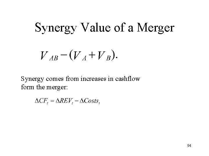
Synergy Value of a Merger Synergy comes from increases in cashflow form the merger: 94

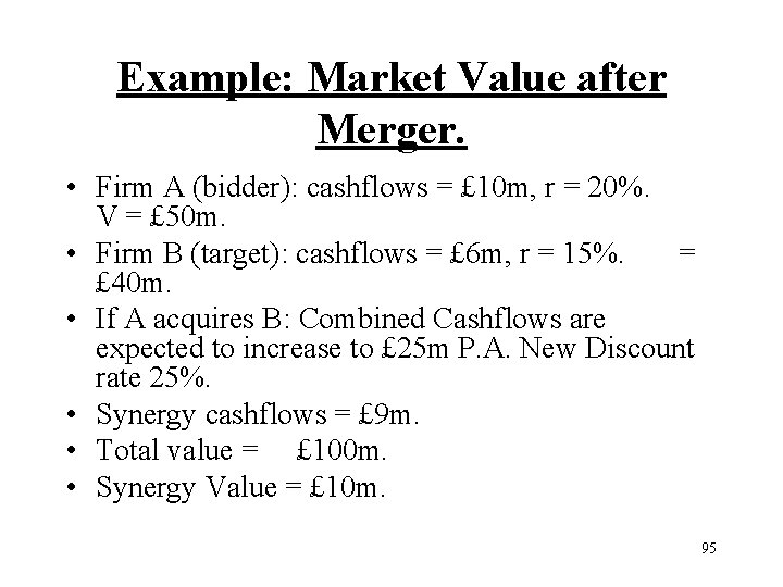
Example: Market Value after Merger. • Firm A (bidder): cashflows = £ 10 m, r = 20%. V = £ 50 m. • Firm B (target): cashflows = £ 6 m, r = 15%. = £ 40 m. • If A acquires B: Combined Cashflows are expected to increase to £ 25 m P. A. New Discount rate 25%. • Synergy cashflows = £ 9 m. • Total value = £ 100 m. • Synergy Value = £ 10 m. 95

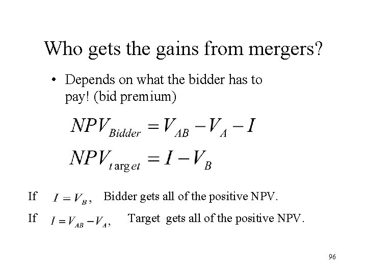
Who gets the gains from mergers? • Depends on what the bidder has to pay! (bid premium) If If Bidder gets all of the positive NPV. Target gets all of the positive NPV. 96

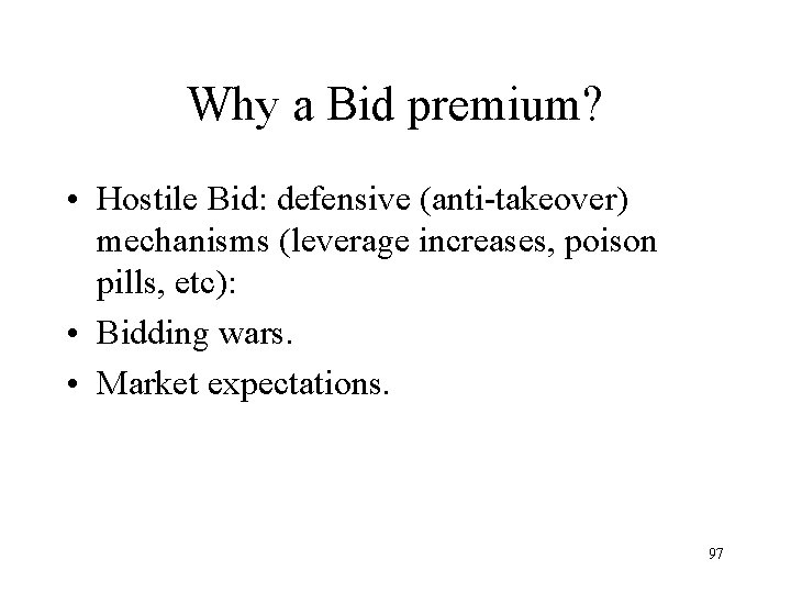
Why a Bid premium? • Hostile Bid: defensive (anti-takeover) mechanisms (leverage increases, poison pills, etc): • Bidding wars. • Market expectations. 97

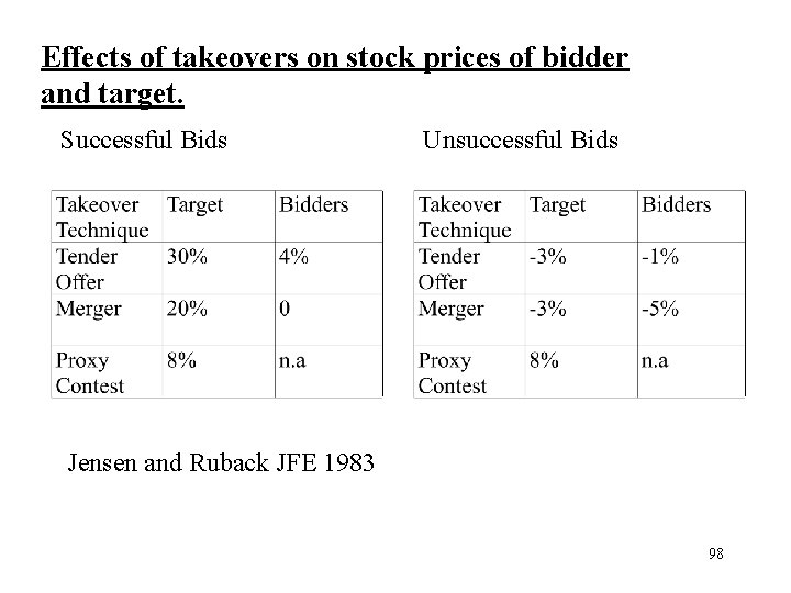
Effects of takeovers on stock prices of bidder and target. Successful Bids Unsuccessful Bids Jensen and Ruback JFE 1983 98

Game Theoretic Approach to M and A. • Grossman and Hart (Special Issue on Corporate Control 1982). • Harris and Raviv (Special Issue on Corporate Control 1982). • Bebchuk (Special Issue on Corporate Control 1982). . • Burkart (JOF 1995). • Garvey and Hanka. • Krause. 99

Garvey and Hanka paper • Lecture slides to follow. 100

Grossman and Hart free-rider paper • Lecture slides to follow. 101

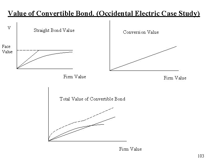
Section 6: Convertible Debt. -Valuation of Convertibles. -Impact on Firm Value. -Why firms issue convertibles. -When are they converted (call policy)? Convertible bond -holder has the right to exchange the bond for common stock (equivalent to a call option). Conversion Ratio = number of shares received for each bond. Value of Convertible Bond = Max{ Straight bond value, 102 Conversion Value} +option value.

Value of Convertible Bond. (Occidental Electric Case Study) V Straight Bond Value Conversion Value Face Value Firm Value Total Value of Convertible Bond Firm Value 103

Conflict between Convertible Bond holders and managers. Convertible Bond = straight debt + call option. Value of a call option increases with: Time. Risk of firm’s cashflows. Implications: Holders of convertible debt maximise value by not converting until forced to do so => Managers will want to force conversion as soon as possible. Incentive for holders to choose risky projects => managers want to choose safe projects. 104

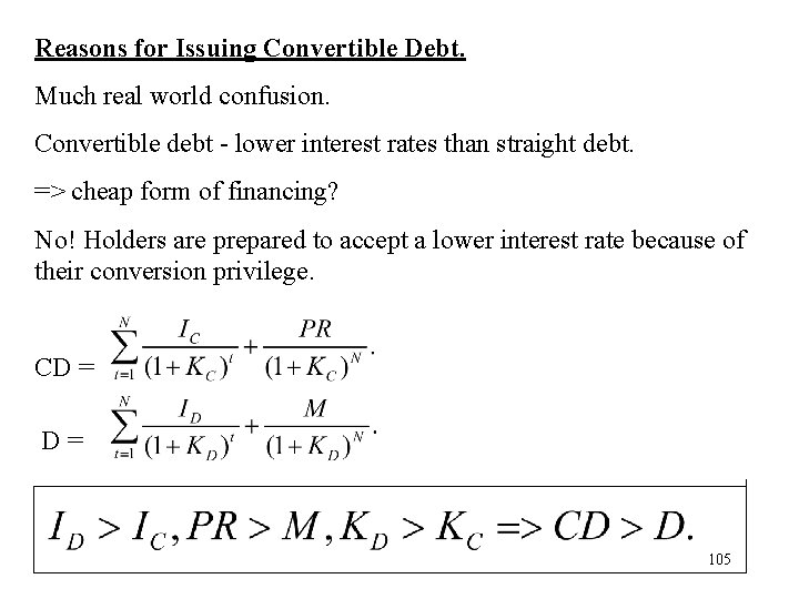
Reasons for Issuing Convertible Debt. Much real world confusion. Convertible debt - lower interest rates than straight debt. => cheap form of financing? No! Holders are prepared to accept a lower interest rate because of their conversion privilege. CD = D= 105

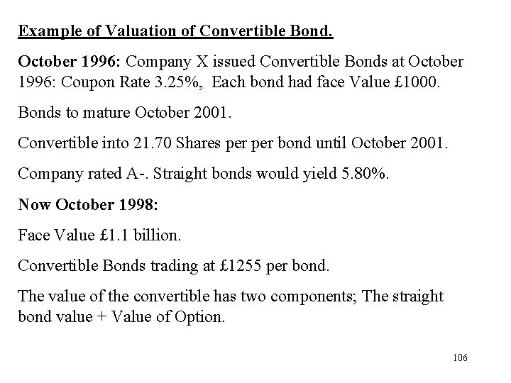
Example of Valuation of Convertible Bond. October 1996: Company X issued Convertible Bonds at October 1996: Coupon Rate 3. 25%, Each bond had face Value £ 1000. Bonds to mature October 2001. Convertible into 21. 70 Shares per bond until October 2001. Company rated A-. Straight bonds would yield 5. 80%. Now October 1998: Face Value £ 1. 1 billion. Convertible Bonds trading at £ 1255 per bond. The value of the convertible has two components; The straight bond value + Value of Option. 106

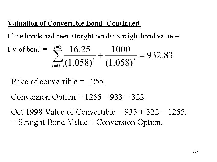
Valuation of Convertible Bond- Continued. If the bonds had been straight bonds: Straight bond value = PV of bond = Price of convertible = 1255. Conversion Option = 1255 – 933 = 322. Oct 1998 Value of Convertible = 933 + 322 = 1255. = Straight Bond Value + Conversion Option. 107

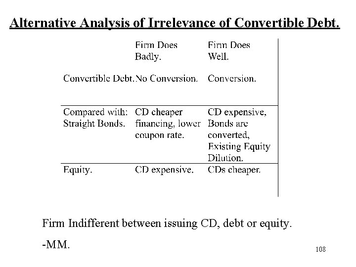
Alternative Analysis of Irrelevance of Convertible Debt. Firm Indifferent between issuing CD, debt or equity. -MM. 108

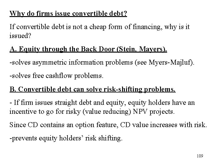
Why do firms issue convertible debt? If convertible debt is not a cheap form of financing, why is it issued? A. Equity through the Back Door (Stein, Mayers). -solves asymmetric information problems (see Myers-Majluf). -solves free cashflow problems. B. Convertible debt can solve risk-shifting problems. - If firm issues straight debt and equity, equity holders have an incentive to go for risky (value reducing) NPV projects. Since CD contains an option feature, CD value increases with risk. -prevents equity holders’ risk shifting. 109

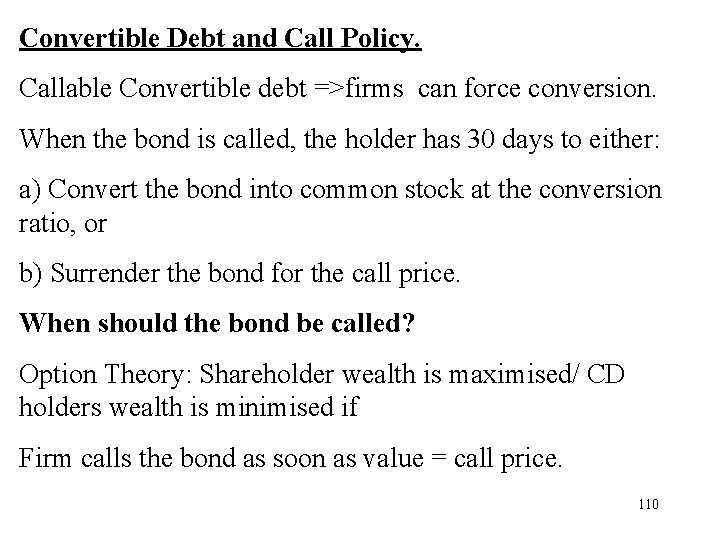
Convertible Debt and Call Policy. Callable Convertible debt =>firms can force conversion. When the bond is called, the holder has 30 days to either: a) Convert the bond into common stock at the conversion ratio, or b) Surrender the bond for the call price. When should the bond be called? Option Theory: Shareholder wealth is maximised/ CD holders wealth is minimised if Firm calls the bond as soon as value = call price. 110

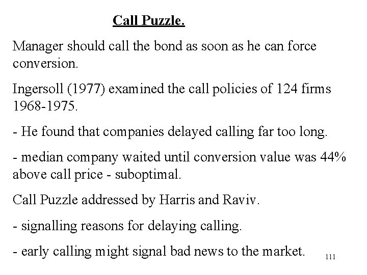
Call Puzzle. Manager should call the bond as soon as he can force conversion. Ingersoll (1977) examined the call policies of 124 firms 1968 -1975. - He found that companies delayed calling far too long. - median company waited until conversion value was 44% above call price - suboptimal. Call Puzzle addressed by Harris and Raviv. - signalling reasons for delaying calling. - early calling might signal bad news to the market. 111