Lecture 17 Regression Diagnostics II More on Residuals

Lecture 17: Regression Diagnostics II More on Residuals

Residuals • Residuals are used to investigate the lack of fit of a model to a given subject • For Cox regression, there’s no easy analog to the usual “observed minus predicted” residuals from linear regression

Regression Diagnostics • We’ve examined how to check the proportional hazards assumption – Graphical approaches – Regression approaches • Time-varying covariates • Schoenfeld residual test • Once we have verified that this assumption is met, we also want to examine – Model goodness of fit – Functional form of covariates – Outliers or influential points

Using Residuals for Diagnostics • Several types – – Schoenfeld residuals (for PH assumption) Cox-Snell residuals Martingale residuals Deviance residuals (similar to Martingale) • What are residuals? – Linear regression: – What is the interpretation of a residual in Cox regression? – Not necessarily the same

Cox-Snell “residuals” • Where – H 0(Tj) = baseline cumulative hazard at time Tj – Zjk is kth covariate value for the jth person – bk is the coefficient estimate for the kth covariate • Interpretation – The expected number of events for each observation • Theory – If model fits, rj’s should look like a censored sample from a unit exponential distribution (i. e. l = 1) – That is, deviations from expected should be small

Why? Some Theory Behind This… •

Why? Some Theory Behind This… • If we define, Y = H(X), as cumulative hazard of X • Then • Thus Y ~ exp(1) regardless of the distribution of X • And so HX(X) should look ~ exp(1)

Cox-Snell Residuals • How do we use these residuals in linear regression? • Assess: – Model fit – Model assumptions • What should we compare Cox-Snell residuals to?

Empirical vs. Fitted • rj = Cox-Snell residuals • CS residuals are always >0 • Hcs(t) = Nelson-Aalen H(t) = empirical cumulative hazard – Estimate by fitting cox model with residuals as time variable and dj as event indicator • If model fits/obeys, i. e. assumptions/covariates are appropriately modeled then: – Plot of rj’s vs. Hcs(t) should be…

Implementation • Get Cox-Snell residuals – – Get linear predictor(s) Zb Get baseline cumulative hazard Multiply OR… get them from R • Get cumulative hazard estimates: – Estimate SNA(t) using KM approach with event time = rj and event indicator = dj – Transform to Hcs(t) scale

Getting Residuals #fit regression reg<-coxph(st~dx+fab+ttrans+mtx+dnage+ptage+dnage*ptage, method="breslow") #get cox-snell residuals par(mfrow=c(1, 2)) cs. res<-event-reg$residuals #Plot of residuals vs. cum hazard fitres<-survfit(coxph(Surv(cs. res, bmt$Either)~1, method="breslow"), type="aalen") plot(fitres$time, -log(fitres$surv), type="s", xlab="Cox-Snell Residuals", ylab="Estimated Cumulative Hazard Function", lwd=2) abline(0, 1, col=2, lwd=2) ## Alternatively, use reg 2<-survfit(Surv(cs. res, bmt$Either)~1) Htilde<-cumsum(reg 2$n. event/reg 2$n. risk) plot(reg 2$time, Htilde, type="s", xlab="Cox-Snell Residuals", ylab="Estimated Cumulative Hazard Function", lwd=2, col=4) abline(0, 1, col=2, lwd=2)

Diagnostic Plots

What about MTX? • Recall MTX did not meet the proportional hazards assumption • Let’s look at each MTX group to see how this effects fit • Also look at MTX stratified model

R Code: MTX Groups cs. res 0<-cs. res[which(bmt$MTX==0)]; event 0<-event[which(bmt$MTX==0)] cs. res 1<-cs. res[which(bmt$MTX==1)]; event 1<-event[which(bmt$MTX==1)] fitres 0<-survfit(coxph(Surv(cs. res 0, event 0)~1, method="breslow"), type="aalen") fitres 1<-survfit(coxph(Surv(cs. res 1, event 1)~1, method="breslow"), type="aalen") plot(fitres 0$time, -log(fitres 0$surv), type="s", xlab="Cox-Snell Residuals", ylab="Estimated Cumulative Hazard Function", col=3, lwd=2, lty=2, xlim=c(0, 3), ylim=c(0, 3)) lines(fitres 1$time, -log(fitres 1$surv), type="s", col=4, lwd=2, lty=2) abline(0, 1, col=2, lwd=2) legend(2, . 5, c("MTX=0", "MTX=1"), col=3: 4, lty=2, lwd=2, bty="n")

R: MTX Groups

R Code: MTX Stratified st<-Surv(dfs, event) reg. strat<-coxph(st~dx+fab+ttrans+dnage+ptage+dnage*ptage+strata(mtx), method="breslow") cs. strat<-event-reg. strat$resid cs. strat 0<-cs. strat[which(bmt$MTX==0)] cs. strat 1<-cs. strat[which(bmt$MTX==1)] fitres. strat 0<-survfit(coxph(Surv(cs. strat 0, event 0)~1, method="breslow"), type="aalen") fitres. strat 1<-survfit(coxph(Surv(cs. strat 1, event 1)~1, method="breslow"), type="aalen") plot(fitres. strat 0$time, -log(fitres. strat 0$surv), type="s", xlab="Cox-Snell Residuals", ylab="Estimated Cumulative Hazard Function", lwd=2, xlim=c(0, 3), ylim=c(0, 3)) lines(fitres. strat 1$time, -log(fitres. strat 1$surv), type="s", col=5, lwd=2) abline(0, 1, col=2, lwd=2) legend(2, . 5, c("MTX=0", "MTX=1"), col=c(1, 5), lwd=2, bty="n")

MTX Stratified Model

Alternative Plots for CS Residuals • There alternative plots you can consider but they tend to require larger N • We can plot: – CS residuals vs. Exp(1) – CS residuals vs. CS-NA cumulative hazard estimate • Let’s consider a larger dataset…

Large Data Set • Study examining factors that impact the time until firsttime mother’s weaned their infants • Data includes information on 927 mothers • Variables in the data include – – – – Race (white, black, other) Mother in poverty Smoking at childbirth Alcohol use at child birth Age of the mother Years of school Prenatal care after the 3 rd month

Model > data(bfeed) > mod<-coxph(Surv(duration, delta)~factor(race)+poverty+smoke+alcohol+agemth+yschool+pc 3 mth, data=bfeed) > mod Call: coxph(formula = Surv(duration, delta) ~ factor(race) + poverty + smoke + yschool + pc 3 mth, data = bfeed) coef exp(coef) se(coef) z p factor(race)2 0. 177 1. 193 0. 1040 1. 70 0. 0890 factor(race)3 0. 306 1. 358 0. 0970 3. 16 0. 0016 poverty -0. 222 0. 801 0. 0929 -2. 39 0. 0170 smoke 0. 249 1. 283 0. 0791 3. 14 0. 0017 alcohol 0. 170 1. 185 0. 1227 1. 38 0. 1700 yschool -0. 040 0. 961 0. 0192 -2. 08 0. 0370 Likelihood ratio test=29. 7 on 6 df, p=4. 51 e-05 n= 927, number of events= 892

CS As Step Function vs. 45 o Line ###Obtaining CS residuals cs. resid<-bfeed$delta-mod$resid ### Fitting Cox model for residuals ### Compare to 450 line fitres<-survfit(coxph(Surv(cs. resid, bfeed$delta)~ 1, method="breslow"), type="aalen") plot(fitres$time, -log(fitres$surv), type="s", xlab="Cox-Snell Residuals", ylab="Estimated Cumulative Hazard Function", lwd=2, ylim=c(0, 8)) abline(0, 1, col=2, lwd=2)

Comparison to Exp(1) ###Obtaining CS residuals cs. resid<-bfeed$delta-mod$resid ### Also compare to exponential efit<-survfit(Surv(duration, delta)~1, data=bfeed) exp 1<-rexp(10000, 1) plot(density(exp 1), lwd=2, col=1) lines(density(cs. resid), col=2, lwd=2, lty=2)

Comparing CS and NA ###Comparing NA to CS NAe<--log(efit$surv) cs<-cbind(cs. resid, bfeed$duration) na<-cbind(NAe, efit$time) all<-merge(cs, na, by=2, all=T) cs<-all$cs. resid[-927] na<-all$NAe[-927] plot(cs, na, pch=16, xlab="Cox-Snell", ylab="Cox-Snell - Nelson-Aalen") abline(0, 1, col=2, lwd=2) fit 1<-lm(na~cs) abline(fit 1, lwd=2, col=3)

Problem with Cox-Snell Approach • CS residuals can diagnose that the model does not fit • But they don’t help figure out why or where • Note, overall pattern can be helpful (e. g. CS > NA or vice versa) • Martingale residuals are better

Martingale Residuals • When model is correct, E(Mj) = 0 • Range between -∞ and 1 • Difference over time between observed and expected number of events – Mj tends to be negative if estimated cumulative hazard is too large – Mj tends to be positive if estimated cumulative hazard is too small

Martingale Residuals • Average martingale can be computed for different values of a covariate – Or range of covariate values – Determines if Mjs tend to be positive or negative in the range • Helps to find improper specification of effect of covariate on hazard

Use of Martingale Residuals • To examine best functional form of the given covariate • Approach: – Assume optimal model is: – – Fit model with only Z* Save Martingale residuals from Z* model Plot Martingale residuals versus Z 1 Use smoother to help find best transformation • Only works on continuous or ordinal variables!

Example ###Martingale Residuals- NHL vs HOD in BMT data(hodg) fit 1<-coxph(Surv(time, delta)~factor(dtype)+factor(gtype)+score+factor(dtype)*factor(gtype), data=hodg) res 1<-fit 1$resid fit 2<-coxph(Surv(time, delta)~factor(dtype)+factor(gtype)+wtime+factor(dtype)*factor(gtype), data=hodg) res 2<-fit 2$resid par(mfrow=c(1, 2)) plot(bmt 2$wait, res 1, xlab="Waiting Time (months)", ylab="Martingale Residuals", pch=16) lines(lowess(bmt 2$wait, res), col=2, lwd=2) lines(bmt 2$wait, lm(res 1~bmt 2$wait), col=4, lwd=2) plot(bmt 2$kar, res 2, xlab="Karnofsky Score", ylab="Martingale Residuals", pch=16) lines(lowess(bmt 2$karn, res), col=2, lwd=2) lines(bmt 2$karn, lm(res 1~bmt 2$wait), col=4, lwd=2)

Martingale Plots

Model with “Inappropriate” Waiting Time > fit<-coxph(Surv(time, cens)~wait+factor(dis)+factor(graft)+karn+ factor(dis)*factor(graft), data=bmt 2) > summary(fit) Call: coxph(formula = Surv(time, cens) ~ wait + factor(dis) + factor(graft) + karn + factor(dis) * factor(graft), data = bmt 2) n= 43, number of events= 26 wait factor(dis)2 factor(graft)2 karn dis*graft coef -0. 01656 2. 76033 0. 63940 -0. 04948 -2. 37093 exp(coef) 0. 98357 15. 8050 1. 89534 0. 95172 0. 09339 se(coef) z Pr(>|z|) 0. 01021 -1. 623 0. 10461 0. 94738 2. 914 0. 00357 ** 0. 59372 1. 077 0. 28151 0. 01242 -3. 984 6. 77 e-05 *** 1. 03548 -2. 290 0. 02204 *

How Do We Find Best Cutpoint? • Want cutoff that gives largest difference between individuals in the two data-defined groups • Clinically chosen value (i. e. what do clinicians find meaningful? • Choose based on data (often good choice) – Contal and O’Quigley • Keep in mind this may bias the model towards inclusion of covariate

Outcome-Oriented Choice • Contal and O’Quigley steps 1. Identify possible unique cut points 2. Construct dichotomized predictor for all cut points 3. Conduct log-rank test for each dichotomized version of the variable 4. Choose cutoff based on largest log-rank statistic • Based on this procedure, waiting time of 84 months is “best” cut point

Model with Dichotomized Waiting Time > #Model with dichotomized waiting time > iwait<-ifelse(84<=bmt 2$wait, 1, 0) > fit. d<-coxph(Surv(time, cens)~iwait+factor(dis)+factor(graft)+karn+ + factor(dis)*factor(graft), data=bmt 2) > summary(fit. d) Call: coxph(formula = Surv(time, cens) ~ iwait + factor(dis) + factor(graft) + karn + factor(dis) * factor(graft), data = bmt 2) n= 43, number of events= 26 iwait factor(dis)2 factor(graft)2 karn dis: graft coef -2. 05982 2. 32733 0. 66509 -0. 05504 -2. 06684 exp(coef) 0. 12748 10. 25050 1. 94467 0. 94644 0. 12658 se(coef) 1. 05066 0. 73324 0. 59432 0. 01234 0. 92577 z -1. 961 3. 174 1. 119 -4. 459 -2. 233 Pr(>|z|) 0. 0499 * 0. 0015 ** 0. 2631 8. 23 e-06 *** 0. 0256 * *NOTE: we can not use the p-value for our waiting time indicator. We should adjust for multiple comparisons because we consider MANY cut points for waiting time (pg. 273 in text). -Here the adjusted p-value is 0. 679

What About Other Transformations • Mayo Clinic trial in primary biliary cirrhosis (PBC) of the liver (1974 to 1984) • 312 PCB randomized to placebo or D-penicillamine • Clinical, biochemical, and histologic measures also collected • Goal: – develop natural history model (ignoring treatment) to determine how baseline status impacts survival

PCB Survival

PBC Example • Covariates of interest – – – Age Albumin Prothrombin time (i. e. clotting time) Presence of edema Serum bilirubin (mg/d. L) • Edema is a factor variable and is used “as is” • What about the other variables?

Where to Start 1. Fit a model with age and edema 2. Get the martingale residuals from this fit 3. Plot the martingale residuals -vs. age -vs. albumin -vs. bilirubin -vs. prothrombin time 4. Check possible transformations where necessary

Age

Albumin

Bilirubin

The Problem Child… Clotting Time

The Problem Child… Clotting Time • Log transformation is a good first guess but it doesn’t always work • Deviations in the plot don’t necessarily lead us easily to the best functional form • There are many we can try – Z×log(Z) – exp{Z} – Power transformations (think Box-Cox) • So let’s “explore” a little

Try Z×ln. Z and e. Z

Power Transformations?

Power Transformations?

The Point? • Sometimes it is difficult to find a good transformation • Choose among the set of possibilities – Is one transformation more interpretable? – Does a particular transformation make clinical sense? • Add log(bilirubin) and log(albumin) to the model with age and edema to see if this helps

Model and Residuals > ### Model including bilirubin and albumin > fit<-coxph(Surv(time, status)~age + factor(edema)+log(bili)+log(albumin)) > summary(fit) Call: coxph(formula = Surv(time, status) ~ age + factor(edema) + log(bili) + log(albumin)) n= 393, number of events= 161 age factor(edema)0. 5 factor(edema)1 log(bili) log(albumin) > res 1<-fit$resid coef 0. 036521 0. 282970 1. 051715 0. 928080 -2. 716231 exp(coef) 1. 037196 1. 327065 2. 862556 2. 529648 0. 066123 se(coef) 0. 007777 0. 225888 0. 287048 0. 083925 0. 648245 z 4. 696 1. 253 3. 664 11. 058 -4. 190 Pr(>|z|) 2. 65 e-06 *** 0. 210315 0. 000248 *** < 2 e-16 *** 2. 79 e-05 ***

Looking Again at Clotting Time ### Model with JUST age and edema fit<-coxph(Surv(time, status)~age + factor(edema)) plot(protime, res 1, xlab="Clot Time", ylab="Martingale Residuals", pch=16, main="Model w/ Age & Edema") lines(lowess(protime, res 1), col=2, lwd=2) lines(protime, fitted(lm(res 1~protime)), col=4, lwd=4) ### Model including bilirubin and albumin fit<-coxph(Surv(time, status)~age + factor(edema)+log(bili)+log(albumin)) res 2<-resid(fit, type="martingale") plot(protime, res 2, xlab="Clotting Time", ylab="Martingale Residuals", pch=16, main="Model with 4 covariates") lines(lowess(protime, res 2), col=2, lwd=2) lines(protime, fitted(lm(res 2~protime)), col=4, lwd=4)

Compare Residual Plots

Transformations in the Models?

Transformations in the Models?

Transformations in the Models?

What to Conclude? • Transformations better but still not great > pt 1. 5<- (protime)^(-1. 5) > fit<-coxph(Surv(time, status)~age + factor(edema)+log(bili)+log(albumin)+pt 1. 5) > fit Call: coxph(formula = Surv(time, status) ~ age + factor(edema) + log(bili) + log(albumin) + pt 1. 5) coef age 0. 0201 factor(edema)0. 5 0. 1424 factor(edema)1 0. 8580 log(bili) 0. 8652 log(albumin) -2. 896 pt 1. 5 -55. 23 exp(coef) 1. 02 e+00 1. 33 e+00 2. 46 e+00 2. 31 e+00 7. 19 e-02 4. 90 e-21 se(coef) z 0. 00723 3. 28 0. 21378 1. 32 0. 28150 3. 20 0. 07702 10. 86 0. 60271 -4. 37 20. 35634 -2. 30 p 0. 0132 0. 5857 0. 0039 < 2 e-16 2. 7 e-05 0. 0362 Likelihood ratio test=229 on 6 df, p=0 n= 418, number of events= 186

Concerns with Martingale Residuals? • One problem with Martingale residuals… they tend to be asymmetric • Range from -∞ to 1 • These are therefore best used to assess covariate form, NOT general goodness of fit. • Also note, there is susceptibility to overfitting when playing around with functional form

Outliers • Defined in survival as – an unusual observed failure time given the covariate value Zj • Martingale residuals do measure the degree to which the jth subject is an outlier • BUT as we mentioned the distribution is heavily skewed • Makes it hard to identify outliers

Deviance Residuals • Deviance residuals are transformation of Martingale residuals • Better behaved than Martingale residuals – More like ~ N(0, 1) • Helpful for determining outliers • Negative for survival times that are smaller than expected

Deviance vs. Martingale Residuals • Deviance residuals have shorter left and longer right tails • Distribution more closely resembles ~N(0, 1) • Because deviance residuals ~N, we can think of outliers as values outside the range – (-3, 3) – More conservative? (-2. 5, 2. 5)

Compare to ~ N(0, 1) ################## ### DEVIANCE RESIDUALS #################### fit 2<-coxph(Surv(time, delta) ~ factor(dtype) + factor(gtype) + score + wtime + factor(dtype)*factor(gtype), data=hodg) #Comparing Density of Martingale and deviance residuals to ~N(0, 1) par(mfrow=c(1, 2)) mart. res<-resid(fit 2, type="martingale") plot(density(mart. res), main="Martingale Residuals", lwd=2) lines(seq(-3, 3, 0. 1), dnorm(seq(-3, 3, 0. 1)), col=2, lwd=2) dev. res<-resid(fit 2, type="deviance") plot(density(dev. res), main="Deviance Redisduals", lwd=2, ylim=c(0, 0. 4)) lines(seq(-3, 3, 0. 1), dnorm(seq(-3, 3, 0. 1)), col=2, lwd=2)

Compare to ~ N(0, 1)

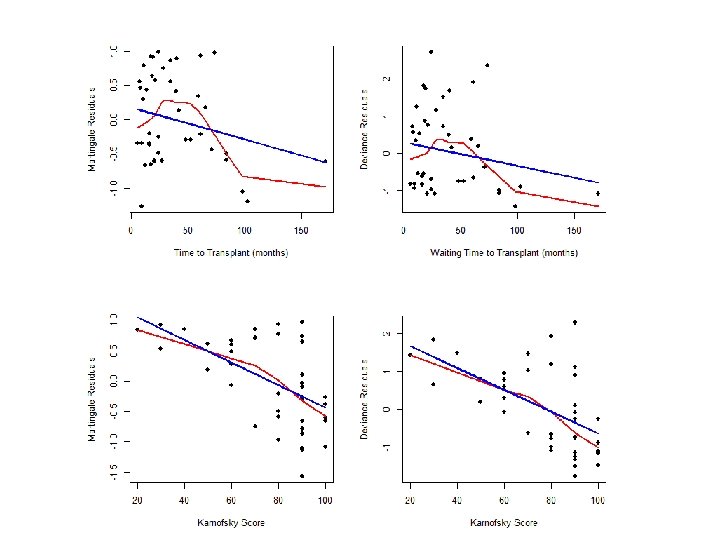
Martingale vs. Deviance Residuals #### Compare deviance to martingale residuals par(mfrow=c(2, 2)) fit 1<-coxph(Surv(time, delta)~factor(dtype)+factor(gtype)+score+factor(dtype)*factor(gtype), data=hodg) mart. res<-resid(fit 1, type="martingale") plot(hodg$wtime, mart. res, xlab="Time to Transplant (months)", ylab="Martingale Residuals", pch=16) lines(lowess(hodg$wtime, mart. res), col=2, lwd=2) lines(hodg$wtime, fitted(lm(mart. res~hodg$wtime)), col=4, lwd=2) dev. res<-resid(fit 1, type="deviance") plot(hodg$wtime, dev. res, xlab="Time to Transplant (months)", ylab="Deviance Residuals", pch=16) lines(lowess(hodg$wtime, dev. res), col=2, lwd=2) lines(hodg$wtime, fitted(lm(dev. res~hodg$wtime)), col=4, lwd=2) fit 2<-coxph(Surv(time, delta)~factor(dtype)+factor(gtype)+wtime+factor(dtype)*factor(gtype), data=hodg) mart. res<-resid(fit 2, type="martingale") plot(hodg$score, mart. res, xlab="Karnofsky Score", ylab="Martingale Residuals", pch=16) lines(lowess(hodg$score, mart. res), col=2, lwd=2) lines(hodg$score, fitted(lm(mart. res~hodg$score)), col=4, lwd=2) dev. res<-resid(fit 2, type="deviance") plot(hodg$score, dev. res, xlab="Karnofsky Score", ylab="Deviance Residuals", pch=16) lines(lowess(hodg$score, dev. res), col=2, lwd=2) lines(hodg$score, fitted(lm(dev. res~hodg$score)), col=4, lwd=2)

Back to Outliers • In order to uses our deviance residuals to determine potential outliers – Plot Dj versus the risk score, • Again, anything outside of (-3, 3) or even more conservative…

R Code > fit<-coxph(Surv(time, status) ~ age + factor(edema) + log(bili) + log(albumin)) > fit Call: coxph(formula = Surv(time, status) ~ age + factor(edema) + log(bili) + log(albumin)) age factor(edema)0. 5 factor(edema)1 log(bili) log(albumin) coef 0. 02209 0. 20292 1. 03318 0. 91211 -2. 91754 exp(coef) 1. 02234 1. 22497 2. 81000 2. 48956 0. 05407 se(coef) 0. 00807 0. 26017 0. 28949 0. 09171 0. 69495 z 2. 74 0. 78 3. 57 9. 95 -4. 20 p 0. 00618 0. 43542 0. 00036 < 2 e-16 2. 7 e-05 Likelihood ratio test=190 on 5 df, p=0, n= 312, number of events= 144 > dev. res<-resid(fit, type="deviance") > lp<-predict(fit, type="lp") > plot(lp, dev. res, xlab=“Risk Score", ylab="Deviance Residual", pch=16) > abline(h=c(-2. 5, 2. 5), col="red", lwd=2) > abline(h=c(-3, 3), col=4, lwd=2)

Outlier Plot

Investigating Outliers > summary(dev. res) Min. 1 st Qu. Median Mean 3 rd Qu. Max. -2. 68587 -0. 71444 -0. 43480 -0. 01337 0. 92603 3. 06954 > summary(cbind(time, status, age, log(albumin), log(bili), edema)) time status age log(albumin) Min. : 41 Min. : 0. 000 Min. : 26. 28 Min. : 0. 6729 1 st Qu. : 1093 1 st Qu. : 0. 000 1 st Qu. : 42. 83 1 st Qu. : 1. 1763 Median : 1730 Median : 0. 000 Median : 51. 00 Median : 1. 2613 Mean : 1918 Mean : 0. 445 Mean : 50. 74 Mean : 1. 2442 3 rd Qu. : 2614 3 rd Qu. : 1. 000 3 rd Qu. : 58. 24 3 rd Qu. : 1. 3271 Max. : 4795 Max. : 1. 000 Max. : 78. 44 Max. : 1. 5347 log(bili) Min. : -1. 2040 1 st Qu. : -0. 2231 Median : 0. 337 Mean : 0. 5715 3 rd Qu. : 1. 2238 Max. : 3. 3322 edema Min. : 1. 000 1 st Qu. : 1. 000 Median : 1. 000 Mean : 1. 201 3 rd Qu. : 1. 000 Max. : 3. 000

Investigating Outliers > cbind(dev. res, cbind(time, status, age, log(albumin), log(bili), edema)) [abs(dev. res) >= 2. 5, ] dev. res time status age log(alb) log(bili) edema 87 3. 0695 198 1 37. 28 1. 482 0. 09531018 1 103 2. 5049 110 1 48. 96 1. 300 0. 91629073 3 119 2. 6630 515 1 54. 26 1. 343 -0. 51082562 1 293 -2. 6859 1320 0 57. 20 1. 092 2. 14006616 3

Caveat with Deviance Residuals • As we’ve seen, deviance residuals can be helpful for identifying outliers • However, given that we are assuming a normal approximation for our residuals, we need to think about sample size • In data with a large number of censored observations (>25%), deviance residuals will tend to be too large.

Influence • Consider only fixed-time covariates • High leverage – An unusual observation with respect to the covariate vector Zi • High influence – An observation for which the combination • Degree to which it is an outlier • And its leverage • = strong influence on estimates of b

Delta-Betas • Let be the estimate of from all the data • Let be the estimate of from data with the ith subject removed • Then the delta-beta is • This is a measure the influence for the ith subject on the estimate of

Delta-Betas • However, this is computationally intensive – Fit model n times • There is an approximation that uses score residuals and the estimated variance-covariance matrix to calculate • Each subject has one model for each covariate in the

Assessing Influence > ### A look at delta-betas for influential points > fit<-coxph(Surv(time, status)~age + factor(edema)+log(bili)+log(albumin)) > dfbeta<-residuals(fit, type="dfbeta") > colnames(dfbeta)<-names(fit$coef) > head(round(dfbeta, 5)) age edema=0. 5 edema=1 log(bili) log(albumin) 1 -0. 00013 0. 00375 -0. 01835 -0. 00146 0. 01982 2 -0. 00035 0. 00173 -0. 00338 0. 00154 -0. 04593 3 0. 00092 0. 04690 0. 01680 -0. 00756 0. 05147 4 0. 00012 -0. 00517 0. 00113 0. 00422 -0. 00757 5 -0. 00063 -0. 00251 -0. 00223 0. 00301 -0. 00251 6 0. 00075 -0. 00403 0. 00382 -0. 00403 0. 02836

Influence Plots >plot(pbc$id[-ids], dfbeta[, 4], xlab="Patient ID", ylab="log(bilirubin) delta-beta", pch=16) > pbc[ dfbeta[, "log(bili)"] < -. 029, c(1, 2, 3, 5, 10, 11, 13)] id time status age edema log(bili) 81 2540 1 63. 26 0 2. 67 362 2267 1 49. 00 0 2. 89 log(albumin) 1. 29 1. 11

Assessment of Influence • Subject 81 is older and has high serum bilirubin (2 sd on log scale) • Bilirubin is an important predictor of high risk, but subjects are in the upper 40 th percentile of survival times • We may want to do a sensitivity analysis with and without observations 81 and 362 • BUT unless we have very good reason (i. e. data entry error) to remove 81, we should not delete them

Next Time • Predictions from a Cox PHM