Introduction to Modern Regression From OLS to GPS

Introduction to Modern Regression: From OLS to GPS® to MARS® September 2014 Dan Steinberg Mikhail Golovnya Salford Systems © 2014 Introduction to Modern Regression 1

Course Outline Today’s Topics • • Regression Problem – quick overview Classical OLS/LOGIT – the starting point RIDGE/LASSO/GPS – regularized regression MARS – adaptive non-linear regression Next Week Topics • Regression Trees • GBM – stochastic gradient boosting • ISLE/RULE-LEARNER – model compression Salford Systems © 2014 Introduction to Modern Regression 2

Regression • Regression analysis at least 200 years old • Surely most used predictive modeling technique (including logistic regression) • American Statistical Association reports 18, 900 members • Bureau of Labor Statistics reported more than 22, 000 statisticians in the work force in 2008 in the USA • Many other professionals involved in the sophisticated analysis of data not included in these counts o Statistical specialists in scientific disciplines such as economics, medicine bioinformatics o Machine Learning specialists, ‘Data Scientists’, database experts o Market researchers studying traditional targeted marketing o Web analytics, social media analytics, text analytics • Few of these other researchers will call themselves statisticians but may make extensive use of variations of regression Salford Systems © 2014 Introduction to Modern Regression 3

Regression Challenges • Preparation of data – errors, missing values, etc. • Determination of predictors to include in model o Hundreds, thousands, even tens and hundreds of thousands available • Transformation or coding of predictors o Conventional approaches consider logarithm, power, inverse, etc. . • Detecting and modeling important interactions • Possibly huge number of records o Super large samples render all predictors “significant” • Complexity of underlying relationship • Lack of external knowledge Salford Systems © 2014 Introduction to Modern Regression 4

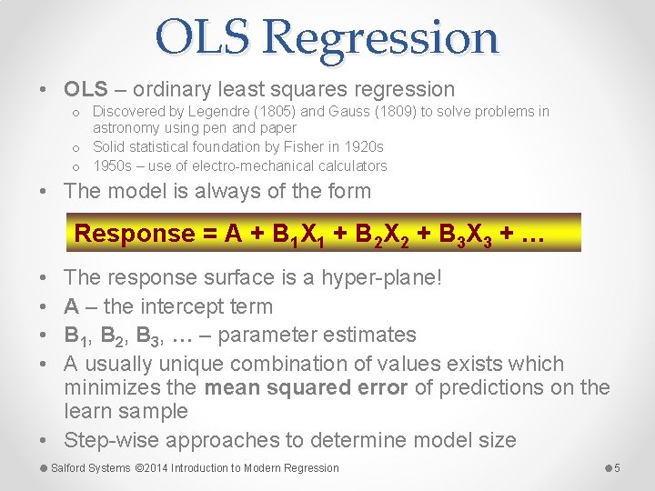
OLS Regression • OLS – ordinary least squares regression o Discovered by Legendre (1805) and Gauss (1809) to solve problems in astronomy using pen and paper o Solid statistical foundation by Fisher in 1920 s o 1950 s – use of electro-mechanical calculators • The model is always of the form Response = A + B 1 X 1 + B 2 X 2 + B 3 X 3 + … • • The response surface is a hyper-plane! A – the intercept term B 1, B 2, B 3, … – parameter estimates A usually unique combination of values exists which minimizes the mean squared error of predictions on the learn sample • Step-wise approaches to determine model size Salford Systems © 2014 Introduction to Modern Regression 5

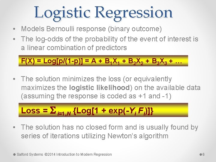
Logistic Regression • Models Bernoulli response (binary outcome) • The log-odds of the probability of the event of interest is a linear combination of predictors F(X) = Log[p/(1 -p)] = A + B 1 X 1 + B 2 X 2 + B 3 X 3 + … • The solution minimizes the loss (or equivalently maximizes the logistic likelihood) on the available data (assuming the response is coded as +1 and -1) Loss = i=1, N {Log[1 + exp(-Yi Fi)]} • The solution has no closed form and is usually found by series of iterations utilizing Newton’s algorithm Salford Systems © 2014 Introduction to Modern Regression 6

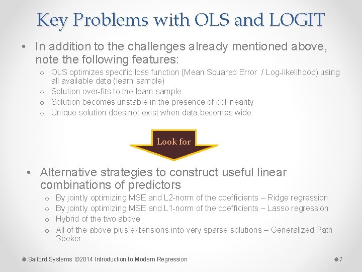
Key Problems with OLS and LOGIT • In addition to the challenges already mentioned above, note the following features: o OLS optimizes specific loss function (Mean Squared Error / Log-likelihood) using all available data (learn sample) o Solution over-fits to the learn sample o Solution becomes unstable in the presence of collinearity o Unique solution does not exist when data becomes wide Look for • Alternative strategies to construct useful linear combinations of predictors o o By jointly optimizing MSE and L 2 -norm of the coefficients – Ridge regression By jointly optimizing MSE and L 1 -norm of the coefficients – Lasso regression Hybrid of the two above All of the above plus extensions into very sparse solutions – Generalized Path Seeker Salford Systems © 2014 Introduction to Modern Regression 7

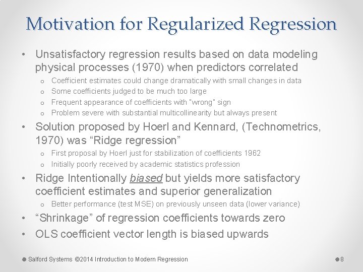
Motivation for Regularized Regression • Unsatisfactory regression results based on data modeling physical processes (1970) when predictors correlated o o Coefficient estimates could change dramatically with small changes in data Some coefficients judged to be much too large Frequent appearance of coefficients with “wrong” sign Problem severe with substantial multicollinearity but always present • Solution proposed by Hoerl and Kennard, (Technometrics, 1970) was “Ridge regression” o First proposal by Hoerl just for stabilization of coefficients 1962 o Initially poorly received by academic statistics profession • Ridge Intentionally biased but yields more satisfactory coefficient estimates and superior generalization o Better performance (test MSE) on previously unseen data (lower variance) • “Shrinkage” of regression coefficients towards zero • OLS coefficient vector length is biased upwards Salford Systems © 2014 Introduction to Modern Regression 8

Lasso Regularized Regression • Introduced by Tibshirani in 1996 explicitly as an improvement on the RIDGE regression • Least Absolute Shrinkage and Selection Operator • Desire to gain the stability and lower variance of ridge regression while also performing variable selection • Especially in the context of many possible predictors looking for a simple, stable, low predictive variance model • Historical note: The Lasso was inspired by related work in 1993 by Leo Breiman (of CART and Random. Forests fame). This was the ‘non-negative garotte’. • Breiman’s simulation studies showed the potential for improved prediction via selection and shrinkage Salford Systems © 2014 Introduction to Modern Regression 9

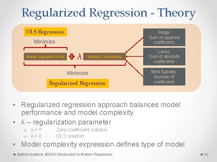
Regularized Regression - Theory OLS Regression Ridge: Sum of squared coefficients Minimize Mean Squared Error λ Model Complexity Minimize Regularized Regression Lasso: Sum of absolute coefficients Best Subsets: Number of coefficients • Regularized regression approach balances model performance and model complexity • λ – regularization parameter o λ = ∞ o λ = 0 Zero-coefficient solution OLS solution • Model complexity expression defines type of model Salford Systems © 2014 Introduction to Modern Regression 10

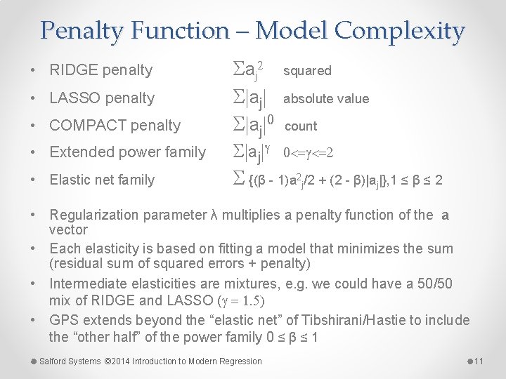
Penalty Function – Model Complexity • RIDGE penalty • LASSO penalty • COMPACT penalty • Extended power family • Elastic net family S a j 2 S|aj|0 S|aj|g squared absolute value count 0<=g<=2 S {(β - 1)a 2 j/2 + (2 - β)|aj|}, 1 ≤ β ≤ 2 • Regularization parameter λ multiplies a penalty function of the a vector • Each elasticity is based on fitting a model that minimizes the sum (residual sum of squared errors + penalty) • Intermediate elasticities are mixtures, e. g. we could have a 50/50 mix of RIDGE and LASSO (g = 1. 5) • GPS extends beyond the “elastic net” of Tibshirani/Hastie to include the “other half” of the power family 0 ≤ β ≤ 1 Salford Systems © 2014 Introduction to Modern Regression 11

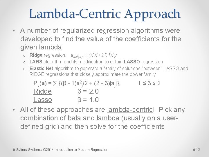
Lambda-Centric Approach • A number of regularized regression algorithms were developed to find the value of the coefficients for the given lambda o Ridge regression: a(ridge) = (X’X +l I)-1 X’y o LARS algorithm and its modification to obtain LASSO regression o Elastic Net algorithm to generate a family of solutions “between” LASSO and RIDGE regressions that closely approximate the power family Pβ(a) = ∑ {(β - 1)a 2 j/2 + (2 - β)|aj|}, 1 ≤ β ≤ 2 Ridge β = 2. 0 Lasso β = 1. 0 • All of these approaches are lambda-centric! Pick any combination of beta and lambda (usually on a userdefined grid) and then solve for the coefficients Salford Systems © 2014 Introduction to Modern Regression 12

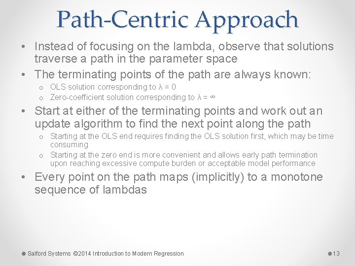
Path-Centric Approach • Instead of focusing on the lambda, observe that solutions traverse a path in the parameter space • The terminating points of the path are always known: o OLS solution corresponding to λ = 0 o Zero-coefficient solution corresponding to λ = ∞ • Start at either of the terminating points and work out an update algorithm to find the next point along the path o Starting at the OLS end requires finding the OLS solution first, which may be time consuming o Starting at the zero end is more convenient and allows early path termination upon reaching excessive compute burden or acceptable model performance • Every point on the path maps (implicitly) to a monotone sequence of lambdas Salford Systems © 2014 Introduction to Modern Regression 13

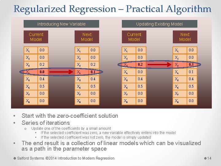
Regularized Regression – Practical Algorithm Introducing New Variable Next Model Current Model • • Next Model Current Model X 1 0. 0 X 2 0. 0 X 3 0. 2 X 3 0. 3 X 4 0. 0 X 4 0. 1 X 5 0. 4 X 6 0. 5 X 7 0. 0 X 8 0. 0 Start with the zero-coefficient solution Series of iterations o • Updating Existing Model Update one of the coefficients by a small amount • If the selected coefficient was zero, a new variable effectively enters into the model • If the selected coefficient was not zero, the model is simply updated The end result is a collection of linear models which can be visualized as a path in the parameter space Salford Systems © 2014 Introduction to Modern Regression 14

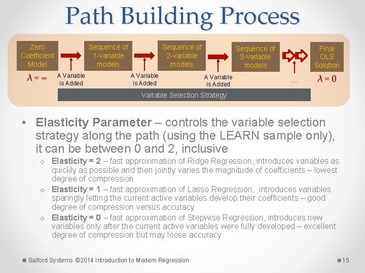
Path Building Process Zero Coefficient Model λ=∞ Sequence of 2 -variable models Sequence of 1 -variable models A Variable is Added Sequence of 3 -variable models A Variable is Added Final OLS Solution … λ=0 Variable Selection Strategy • Elasticity Parameter – controls the variable selection strategy along the path (using the LEARN sample only), it can be between 0 and 2, inclusive o Elasticity = 2 – fast approximation of Ridge Regression, introduces variables as quickly as possible and then jointly varies the magnitude of coefficients – lowest degree of compression o Elasticity = 1 – fast approximation of Lasso Regression, introduces variables sparingly letting the current active variables develop their coefficients – good degree of compression versus accuracy o Elasticity = 0 – fast approximation of Stepwise Regression, introduces new variables only after the current active variables were fully developed – excellent degree of compression but may loose accuracy Salford Systems © 2014 Introduction to Modern Regression 15

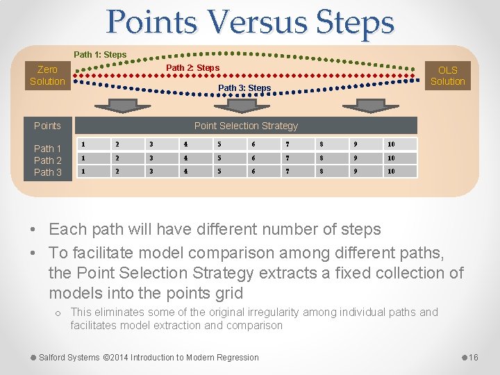
Points Versus Steps Path 1: Steps Path 2: Steps Zero Solution Path 3: Steps Points Path 1 Path 2 Path 3 OLS Solution Point Selection Strategy 1 2 3 4 5 6 7 8 9 10 • Each path will have different number of steps • To facilitate model comparison among different paths, the Point Selection Strategy extracts a fixed collection of models into the points grid o This eliminates some of the original irregularity among individual paths and facilitates model extraction and comparison Salford Systems © 2014 Introduction to Modern Regression 16

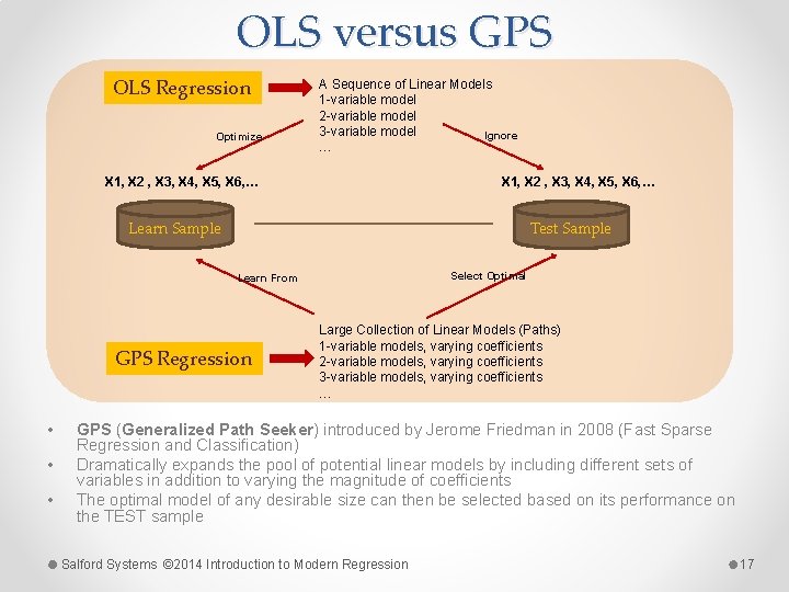
OLS versus GPS OLS Regression Optimize A Sequence of Linear Models 1 -variable model 2 -variable model 3 -variable model Ignore … X 1, X 2 , X 3, X 4, X 5, X 6, … Test Sample Learn Sample Select Optimal Learn From GPS Regression • • • Large Collection of Linear Models (Paths) 1 -variable models, varying coefficients 2 -variable models, varying coefficients 3 -variable models, varying coefficients … GPS (Generalized Path Seeker) introduced by Jerome Friedman in 2008 (Fast Sparse Regression and Classification) Dramatically expands the pool of potential linear models by including different sets of variables in addition to varying the magnitude of coefficients The optimal model of any desirable size can then be selected based on its performance on the TEST sample Salford Systems © 2014 Introduction to Modern Regression 17

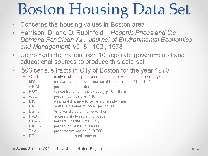
Boston Housing Data Set • Concerns the housing values in Boston area • Harrison, D. and D. Rubinfeld. Hedonic Prices and the Demand For Clean Air. Journal of Environmental Economics and Management, v 5, 81 -102 , 1978 • Combined information from 10 separate governmental and educational sources to produce this data set • 506 census tracts in City of Boston for the year 1970 o o o o Goal: MV CRIM NOX AGE DIS RM LSTAT RAD CHAS INDUS TAX PT study relationship between quality of life variables and property values median value of owner-occupied homes in tract ($1, 000’s) per capita crime rates concentration of nitric oxides (pp 10 million) percent built before 1940 weighted distance to centers of employment average number of rooms per house % lower status of the population accessibility to radial highways borders Charles River (0/1) percent non-retail business property tax rate per $10, 000 pupil teacher ratio Salford Systems © 2014 Introduction to Modern Regression 18

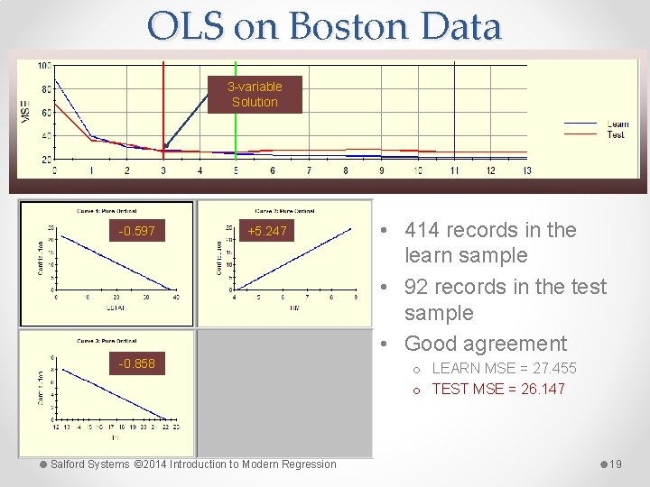
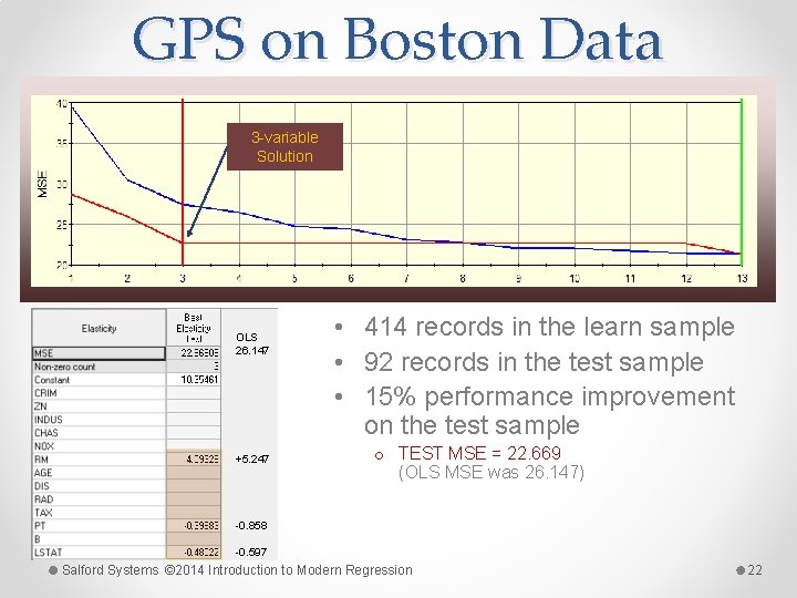
OLS on Boston Data 3 -variable Solution -0. 597 +5. 247 -0. 858 Salford Systems © 2014 Introduction to Modern Regression • 414 records in the learn sample • 92 records in the test sample • Good agreement o LEARN MSE = 27. 455 o TEST MSE = 26. 147 19

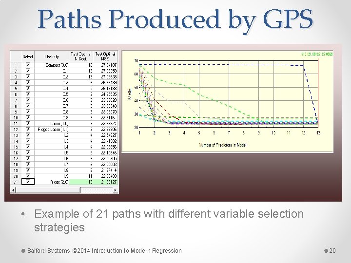
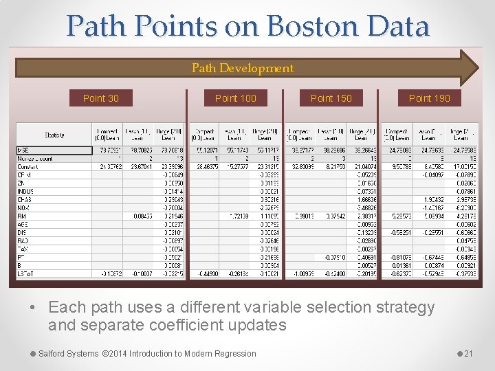
Paths Produced by GPS • Example of 21 paths with different variable selection strategies Salford Systems © 2014 Introduction to Modern Regression 20

Path Points on Boston Data Path Development Point 30 Point 100 Point 150 Point 190 • Each path uses a different variable selection strategy and separate coefficient updates Salford Systems © 2014 Introduction to Modern Regression 21

GPS on Boston Data 3 -variable Solution OLS 26. 147 +5. 247 • 414 records in the learn sample • 92 records in the test sample • 15% performance improvement on the test sample o TEST MSE = 22. 669 (OLS MSE was 26. 147) -0. 858 -0. 597 Salford Systems © 2014 Introduction to Modern Regression 22

Key Problems with GPS • GPS model is still a linear regression! • Response surface is still a global hyper-plane • Incapable of discovering local structure in the data Look for • Develop non-linear algorithms that build response surface locally based on the data itself o By trying all possible data cuts as local boundaries o By fitting first-order adaptive splines locally Salford Systems © 2014 Introduction to Modern Regression 23

Motivation for MARS Multivariate Adaptive Regression Splines • Developed by Jerome H. Friedman in late 1980 s • After his work on CART (for classification) • Adapting many CART ideas for regression o Automatic variable selection o Automatic missing value handling o Allow for nonlinearity o Allow for interactions o Leverage the power of regression where linearity can be exploited Salford Systems © 2014 Introduction to Modern Regression 24

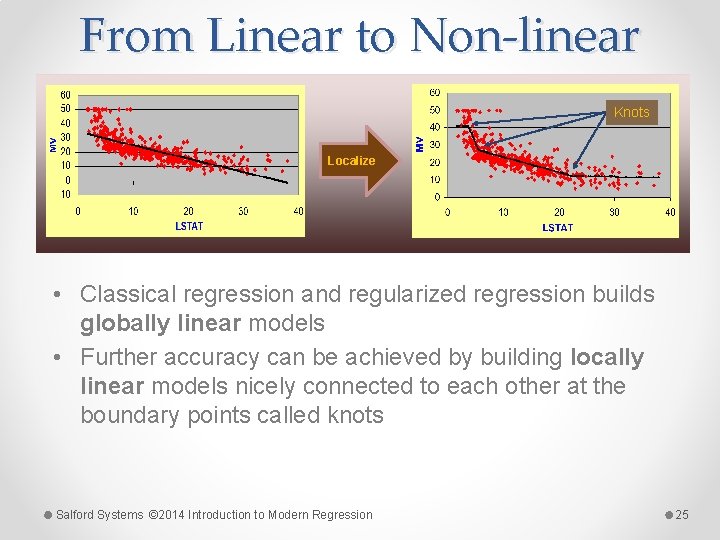
From Linear to Non-linear Knots Localize • Classical regression and regularized regression builds globally linear models • Further accuracy can be achieved by building locally linear models nicely connected to each other at the boundary points called knots Salford Systems © 2014 Introduction to Modern Regression 25

Key Concept for Spline is the “knot” • Knot marks end of one region of data and beginning of another • Knot is where behavior of function changes • In a classical spline knot positions are predetermined and are often evenly spaced • In MARS, knots are determined by search procedure • Only as many knots as needed end up in the MARS model • If a straight line is adequate fit there will be no interior knots o in MARS there is always at least one knot o Could correspond to smallest observed value of the predictor Salford Systems © 2014 Introduction to Modern Regression 26

Placement of Knots • With only one predictor and one knot to select, placement is straightforward: o test every possible knot location o choose model with best fit (smallest SSE) o perhaps constrain by requiring a minimum amount of data in each interval • Prevents interior knot being placed too close to a boundary • For computational efficiency, knots are always placed exactly at observed predictor values o Can cause rare modeling artifacts that sometimes appear due to discrete nature of data Salford Systems © 2014 Introduction to Modern Regression 27

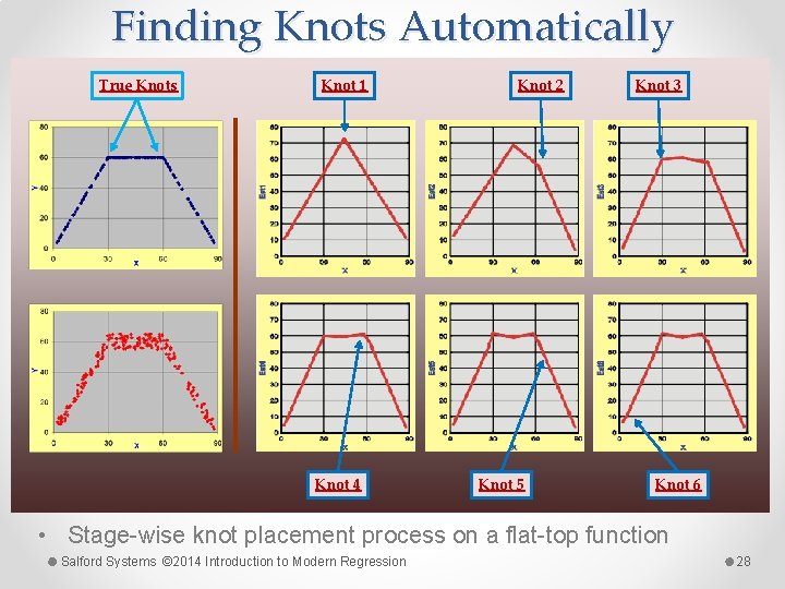
Finding Knots Automatically True Knots Knot 1 Knot 4 Knot 2 Knot 5 Knot 3 Knot 6 • Stage-wise knot placement process on a flat-top function Salford Systems © 2014 Introduction to Modern Regression 28

Basis Functions • Example for knot selection works very well to illustrate splines in one dimension • Thinking in terms of knot locations is unwieldy for working with a large number of variables simultaneously o need a concise notation and programming expressions that are easy to manipulate o Not clear how to construct or represent interactions using knot locations • Basis Functions (BF) provide analytical machinery to express the knot placement strategy • MARS creates sets of basis functions to decompose the information in each variable individually Salford Systems © 2014 Introduction to Modern Regression 29

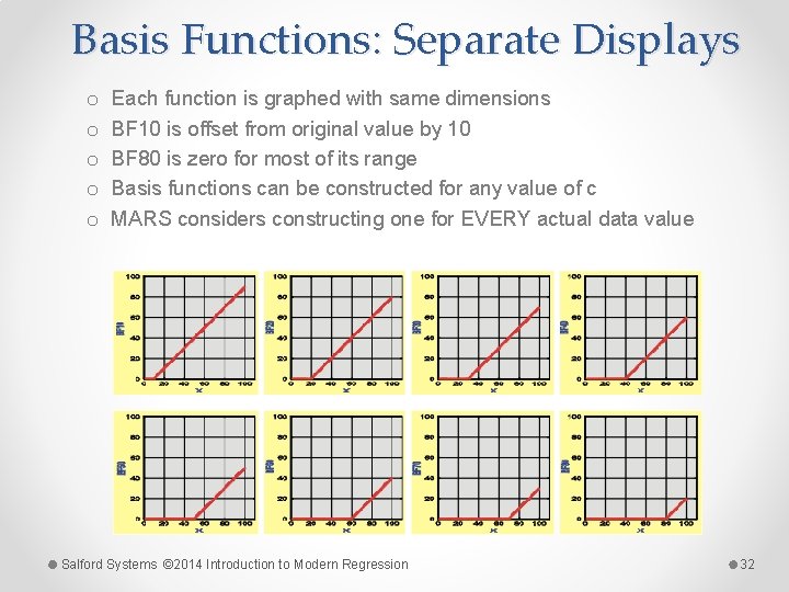
The Hockey Stick Basis Function • Hockey Stick basis function is core MARS building o can be applied to a single variable multiple times • Hockey stick function: o Direct: max (0, X -c) o Mirror: max (0, c - X) o Maps variable X to new variable X* o X* =0 for all values of X up to some threshold value c o X* =X – c for all values of X greater than c • the amount by which X exceeds threshold c Salford Systems © 2014 Introduction to Modern Regression 30

Basis Function Example • X ranges from 0 to 100 • 8 basis functions displayed (c=10, 20, 30, …, 80) Salford Systems © 2014 Introduction to Modern Regression 31

Basis Functions: Separate Displays o o o Each function is graphed with same dimensions BF 10 is offset from original value by 10 BF 80 is zero for most of its range Basis functions can be constructed for any value of c MARS considers constructing one for EVERY actual data value Salford Systems © 2014 Introduction to Modern Regression 32

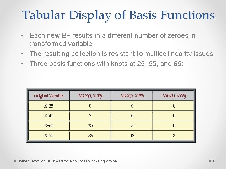
Tabular Display of Basis Functions • Each new BF results in a different number of zeroes in transformed variable • The resulting collection is resistant to multicollinearity issues • Three basis functions with knots at 25, 55, and 65: Salford Systems © 2014 Introduction to Modern Regression 33

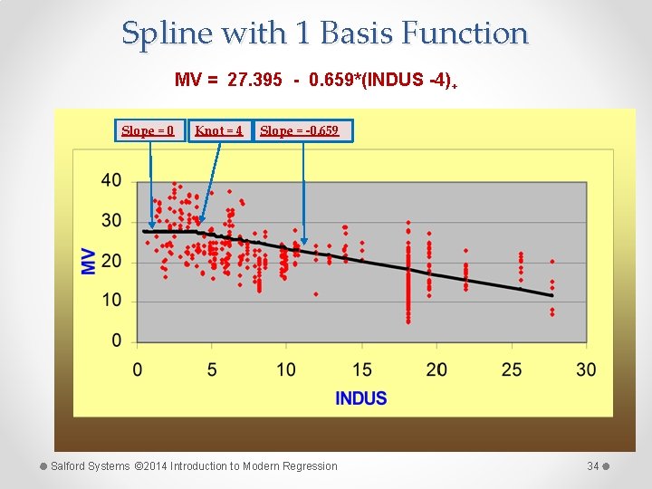
Spline with 1 Basis Function MV = 27. 395 - 0. 659*(INDUS -4)+ Slope = 0 Knot = 4 Slope = -0. 659 Salford Systems © 2014 Introduction to Modern Regression 34

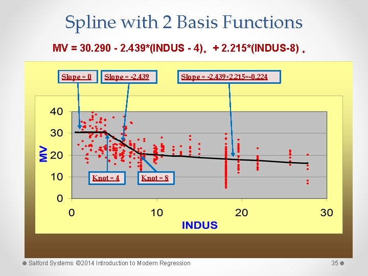
Spline with 2 Basis Functions MV = 30. 290 - 2. 439*(INDUS - 4)+ + 2. 215*(INDUS-8) + Slope = 0 Slope = -2. 439 Knot = 4 Slope = -2. 439+2. 215=-0. 224 Knot = 8 Salford Systems © 2014 Introduction to Modern Regression 35

Adding Mirror Image BF • • A standard basis function (X - knot)+ does not provide for a non-zero slope for values below the knot To handle this MARS uses a “mirror image” basis function, which looks at the interval of a variable X which lies below the threshold c 29. 433 + 0. 925*(4 - INDUS) -2. 180*(INDUS-4) +1. 939*(INDUS-8) MV= + + + Slope = -0. 925 Slope = -2. 180 Knot = 4 Slope = -2. 180+1. 939=-0. 241 Knot = 8 Salford Systems © 2014 Introduction to Modern Regression 36

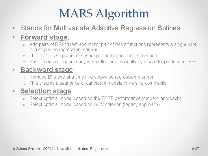
MARS Algorithm • Stands for Multivariate Adaptive Regression Splines • Forward stage: o Add pairs of BFs (direct and mirror pair of basis functions represents a single knot) in a step-wise regression manner o The process stops once a user specified upper limit is reached o Possible linear dependency is handled automatically by discarding redundant BFs • Backward stage: o Remove BFs one at a time in a step-wise regression manner o This creates a sequence of candidate models of varying complexity • Selection stage: o Select optimal model based on the TEST performance (modern approach) o Select optimal model based on GCV criterion (legacy approach) Salford Systems © 2014 Introduction to Modern Regression 37

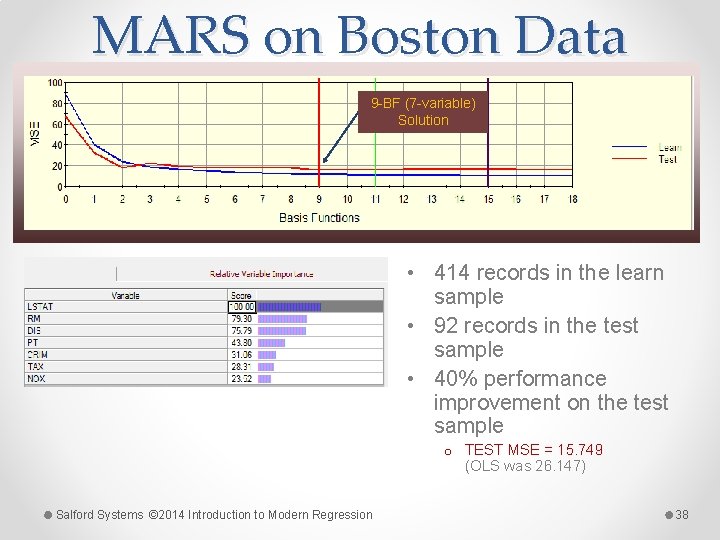
MARS on Boston Data 9 -BF (7 -variable) Solution • 414 records in the learn sample • 92 records in the test sample • 40% performance improvement on the test sample o TEST MSE = 15. 749 (OLS was 26. 147) Salford Systems © 2014 Introduction to Modern Regression 38

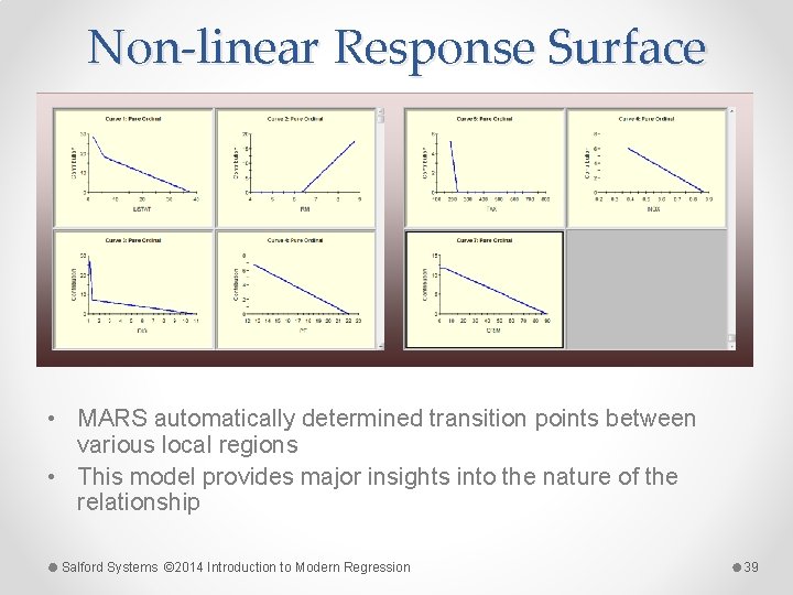
Non-linear Response Surface • MARS automatically determined transition points between various local regions • This model provides major insights into the nature of the relationship Salford Systems © 2014 Introduction to Modern Regression 39

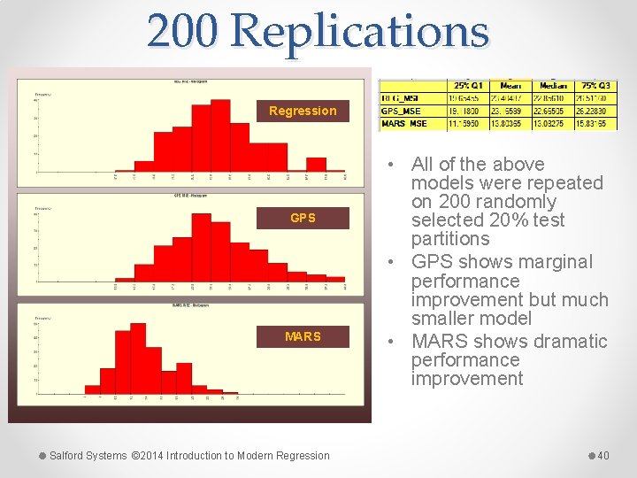
200 Replications Regression GPS MARS Salford Systems © 2014 Introduction to Modern Regression • All of the above models were repeated on 200 randomly selected 20% test partitions • GPS shows marginal performance improvement but much smaller model • MARS shows dramatic performance improvement 40

Regression Trees • Regression trees result to piece-wise constant models (multi-dimensional staircase) on an orthogonal partition of the data space o Thus usually not the best possible performer in terms of conventional regression loss functions • Only a very limited number of controls is available to influence the modeling process o Priors and costs are no longer applicable o There are two splitting rules: LS and LAD • Very powerful in capturing high-order interactions but somewhat weak in explaining simple main effects Salford Systems © 2014 Introduction to Modern Regression 41

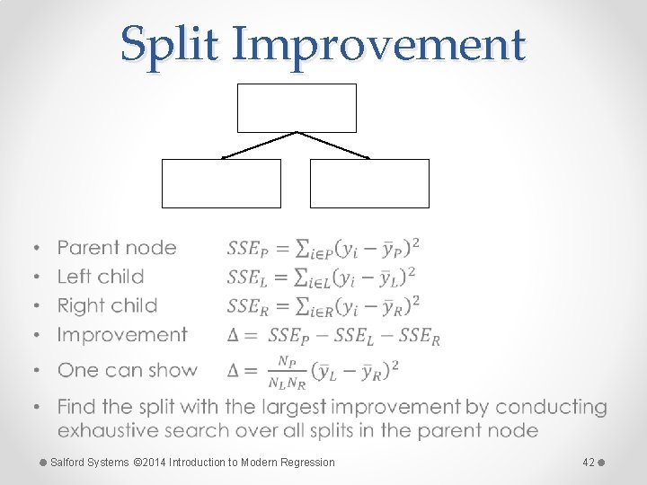
Split Improvement • Salford Systems © 2014 Introduction to Modern Regression 42

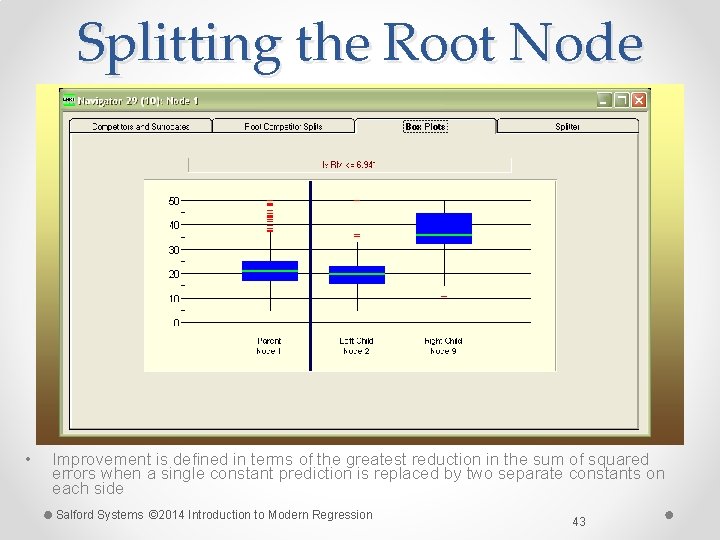
Splitting the Root Node • Improvement is defined in terms of the greatest reduction in the sum of squared errors when a single constant prediction is replaced by two separate constants on each side Salford Systems © 2014 Introduction to Modern Regression 43

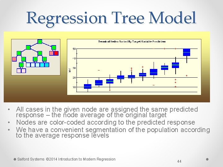
Regression Tree Model • All cases in the given node are assigned the same predicted response – the node average of the original target • Nodes are color-coded according to the predicted response • We have a convenient segmentation of the population according to the average response levels Salford Systems © 2014 Introduction to Modern Regression 44

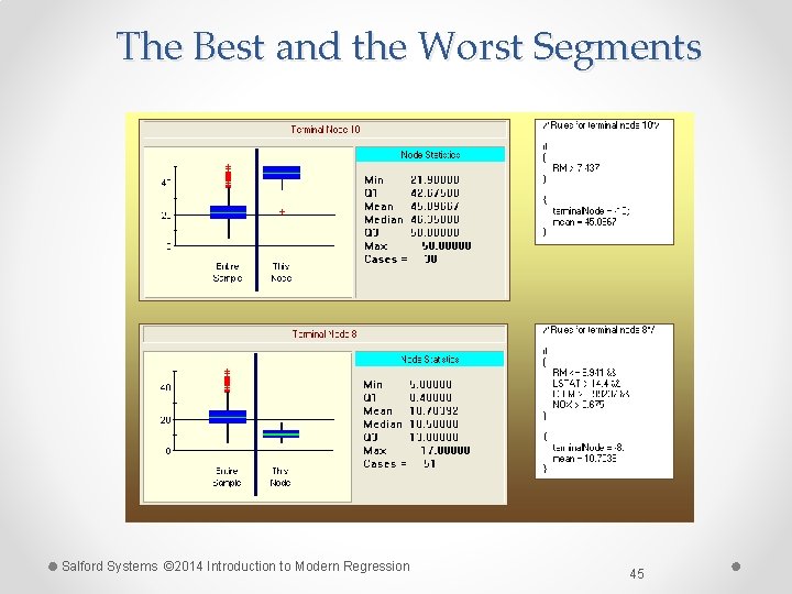
The Best and the Worst Segments Salford Systems © 2014 Introduction to Modern Regression 45

Stochastic Gradient Boosting • New approach to machine learning /function approximation developed by Jerome H. Friedman at Stanford University o Co-author of CART® with Breiman, Olshen and Stone o Author of MARS®, PRIM, Projection Pursuit • Also known as Treenet® • Good for classification and regression problems • Built on small trees and thus o o Fast and efficient Data driven Immune to outliers Invariant to monotone transformations of variables • Resistant to over training – generalizes very well • Can be remarkably accurate with little effort • BUT resulting model may be very complex Salford Systems © 2014 Introduction to Modern Regression 46

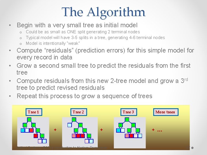
The Algorithm • Begin with a very small tree as initial model o Could be as small as ONE split generating 2 terminal nodes o Typical model will have 3 -5 splits in a tree, generating 4 -6 terminal nodes o Model is intentionally “weak” • Compute “residuals” (prediction errors) for this simple model for every record in data • Grow a second small tree to predict the residuals from the first tree • Compute residuals from this new 2 -tree model and grow a 3 rd tree to predict revised residuals • Repeat this process to grow a sequence of trees Tree 1 Tree 2 + Tree 3 + Salford Systems © 2014 Introduction to Modern Regression More trees + … 47

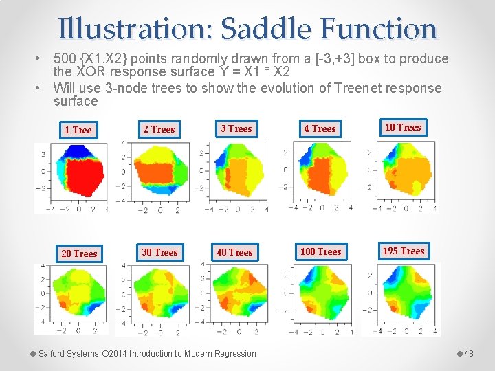
Illustration: Saddle Function • 500 {X 1, X 2} points randomly drawn from a [-3, +3] box to produce the XOR response surface Y = X 1 * X 2 • Will use 3 -node trees to show the evolution of Treenet response surface 1 Tree 2 Trees 3 Trees 4 Trees 10 Trees 20 Trees 30 Trees 40 Trees 100 Trees 195 Trees Salford Systems © 2014 Introduction to Modern Regression 48

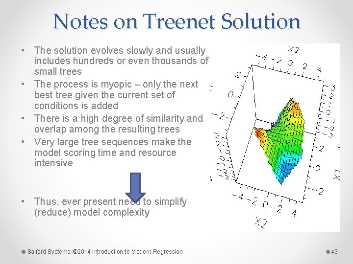
Notes on Treenet Solution • The solution evolves slowly and usually includes hundreds or even thousands of small trees • The process is myopic – only the next best tree given the current set of conditions is added • There is a high degree of similarity and overlap among the resulting trees • Very large tree sequences make the model scoring time and resource intensive • Thus, ever present need to simplify (reduce) model complexity Salford Systems © 2014 Introduction to Modern Regression 49

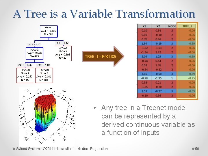
A Tree is a Variable Transformation TREE_1 = F(X 1, X 2) • Any tree in a Treenet model can be represented by a derived continuous variable as a function of inputs Salford Systems © 2014 Introduction to Modern Regression 50

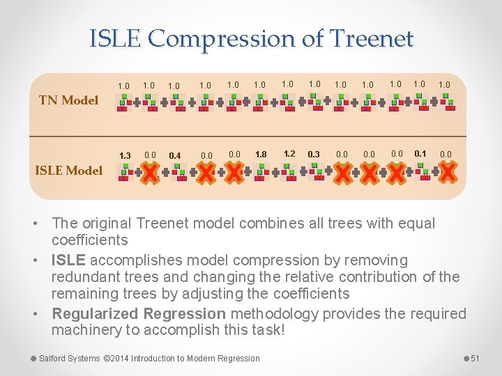
ISLE Compression of Treenet 1. 0 1. 3 0. 0 0. 4 0. 0 1. 8 1. 2 0. 3 0. 0 0. 1 0. 0 TN Model ISLE Model • The original Treenet model combines all trees with equal coefficients • ISLE accomplishes model compression by removing redundant trees and changing the relative contribution of the remaining trees by adjusting the coefficients • Regularized Regression methodology provides the required machinery to accomplish this task! Salford Systems © 2014 Introduction to Modern Regression 51

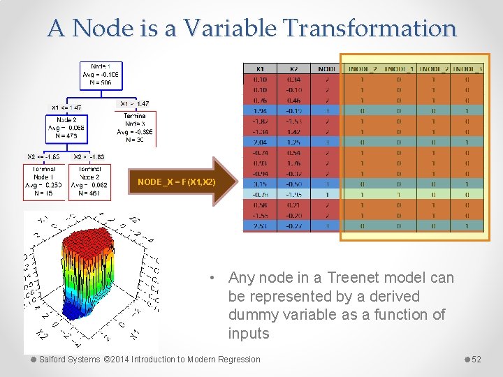
A Node is a Variable Transformation NODE_X = F(X 1, X 2) • Any node in a Treenet model can be represented by a derived dummy variable as a function of inputs Salford Systems © 2014 Introduction to Modern Regression 52

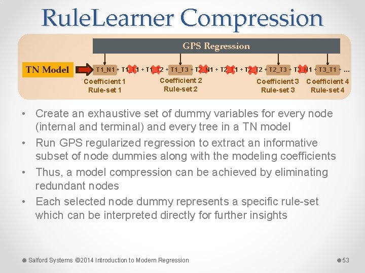
Rule. Learner Compression GPS Regression TN Model T 1_N 1 + T 1_T 2 + T 1_T 3 + T 2_N 1 + T 2_T 2 + T 2_T 3 + T 3_N 1 + T 3_T 1 + … Coefficient 1 Rule-set 1 Coefficient 2 Rule-set 2 Coefficient 3 Rule-set 3 Coefficient 4 Rule-set 4 • Create an exhaustive set of dummy variables for every node (internal and terminal) and every tree in a TN model • Run GPS regularized regression to extract an informative subset of node dummies along with the modeling coefficients • Thus, a model compression can be achieved by eliminating redundant nodes • Each selected node dummy represents a specific rule-set which can be interpreted directly for further insights Salford Systems © 2014 Introduction to Modern Regression 53

Salford Predictive Modeler SPM • Download a current version from our website http: //www. salford-systems. com • Version will run without a license key for 10 -days • Request a license key from unlock@salford-systems. com • Request configuration to meet your needs o Data handling capacity o Data mining engines made available Salford Systems © 2014 Introduction to Modern Regression 54