Chapter 11 Further Issues in Using OLS with

Chapter 11 Further Issues in Using OLS with Time Series Data © 2016 Cengage Learning®. May not be scanned, copied or duplicated, or posted to a publicly accessible website, in whole or in part, except for use as permitted in a license distributed with a certain product or service or otherwise on a password-protected website or school-approved learning management system for classroom use. © kentoh/Shutterstock.

Further Issues in Using OLS with Time Series Data ● The assumptions used so far seem to be too restricitive • Strict exogeneity, homoskedasticity, and no serial correlation are very demanding requirements, especially in the time series context • Statistical inference rests on the validity of the normality assumption • Much weaker assumptions are needed if the sample size is large • A key requirement for large sample analysis of time series is that the time series in question are stationary and weakly dependent ● Stationary time series • Loosely speaking, a time series is stationary if its stochastic properties and its temporal dependence structure do not change over time © 2016 Cengage Learning®. May not be scanned, copied or duplicated, or posted to a publicly accessible website, in whole or in part, except for use as permitted in a license distributed with a certain product or service or otherwise on a password-protected website or school-approved learning management system for classroom use.

Further Issues in Using OLS with Time Series Data ● Stationary stochastic processes A stochastic process is stationary, if for every collection of indices the joint distribution of , is the same as that of for all integers . ● Covariance stationary processes A stochastic process is covariance stationary, if its expected value, its variance, and its covariances are constant over time: 1) , 2) , and 3) © 2016 Cengage Learning®. May not be scanned, copied or duplicated, or posted to a publicly accessible website, in whole or in part, except for use as permitted in a license distributed with a certain product or service or otherwise on a password-protected website or school-approved learning management system for classroom use. .

Further Issues in Using OLS with Time Series Data ● Weakly dependent time series A stochastic process “almost independent” of is weakly dependent , if if is grows to infinity (for all ). ● Discussion of the weak dependence property • An implication of weak dependence is that the correlation between , and must converge to zero if grows to infinity • For the LLN and the CLT to hold, the individual observations must not be too strongly related to each other; in particular their relation must become weaker (and this fast enough) the farther they are apart • Note that a series may be nonstationary but weakly dependent © 2016 Cengage Learning®. May not be scanned, copied or duplicated, or posted to a publicly accessible website, in whole or in part, except for use as permitted in a license distributed with a certain product or service or otherwise on a password-protected website or school-approved learning management system for classroom use.

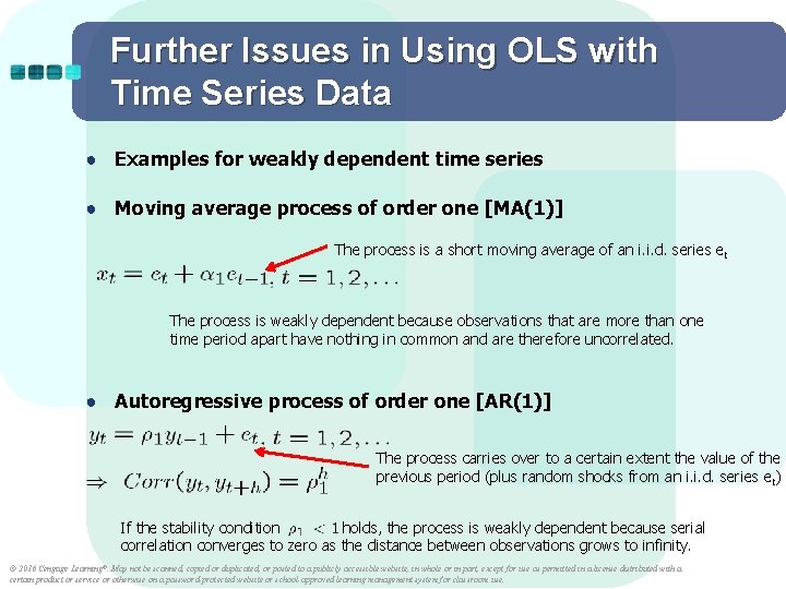
Further Issues in Using OLS with Time Series Data ● Examples for weakly dependent time series ● Moving average process of order one [MA(1)] The process is a short moving average of an i. i. d. series e t The process is weakly dependent because observations that are more than one time period apart have nothing in common and are therefore uncorrelated. ● Autoregressive process of order one [AR(1)] The process carries over to a certain extent the value of the previous period (plus random shocks from an i. i. d. series e t) If the stability condition holds, the process is weakly dependent because serial correlation converges to zero as the distance between observations grows to infinity. © 2016 Cengage Learning®. May not be scanned, copied or duplicated, or posted to a publicly accessible website, in whole or in part, except for use as permitted in a license distributed with a certain product or service or otherwise on a password-protected website or school-approved learning management system for classroom use.

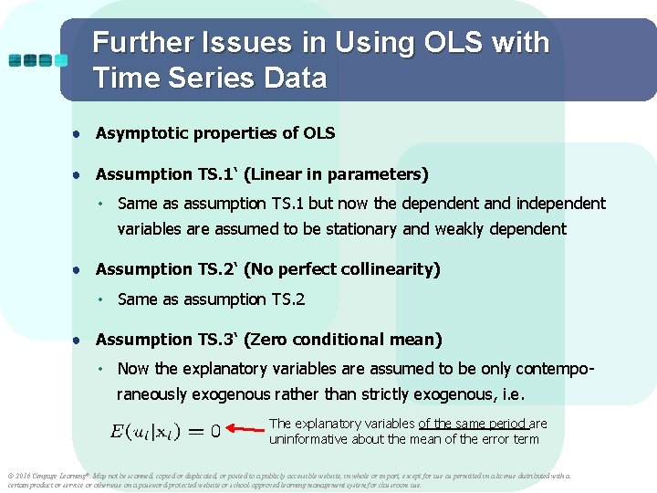
Further Issues in Using OLS with Time Series Data ● Asymptotic properties of OLS ● Assumption TS. 1‘ (Linear in parameters) • Same as assumption TS. 1 but now the dependent and independent variables are assumed to be stationary and weakly dependent ● Assumption TS. 2‘ (No perfect collinearity) • Same as assumption TS. 2 ● Assumption TS. 3‘ (Zero conditional mean) • Now the explanatory variables are assumed to be only contemporaneously exogenous rather than strictly exogenous, i. e. The explanatory variables of the same period are uninformative about the mean of the error term © 2016 Cengage Learning®. May not be scanned, copied or duplicated, or posted to a publicly accessible website, in whole or in part, except for use as permitted in a license distributed with a certain product or service or otherwise on a password-protected website or school-approved learning management system for classroom use.

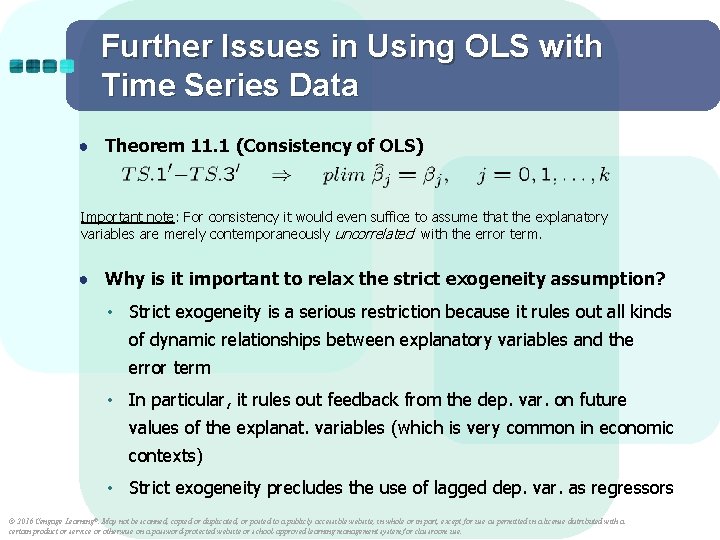
Further Issues in Using OLS with Time Series Data ● Theorem 11. 1 (Consistency of OLS) Important note: For consistency it would even suffice to assume that the explanatory variables are merely contemporaneously uncorrelated with the error term. ● Why is it important to relax the strict exogeneity assumption? • Strict exogeneity is a serious restriction because it rules out all kinds of dynamic relationships between explanatory variables and the error term • In particular, it rules out feedback from the dep. var. on future values of the explanat. variables (which is very common in economic contexts) • Strict exogeneity precludes the use of lagged dep. var. as regressors © 2016 Cengage Learning®. May not be scanned, copied or duplicated, or posted to a publicly accessible website, in whole or in part, except for use as permitted in a license distributed with a certain product or service or otherwise on a password-protected website or school-approved learning management system for classroom use.

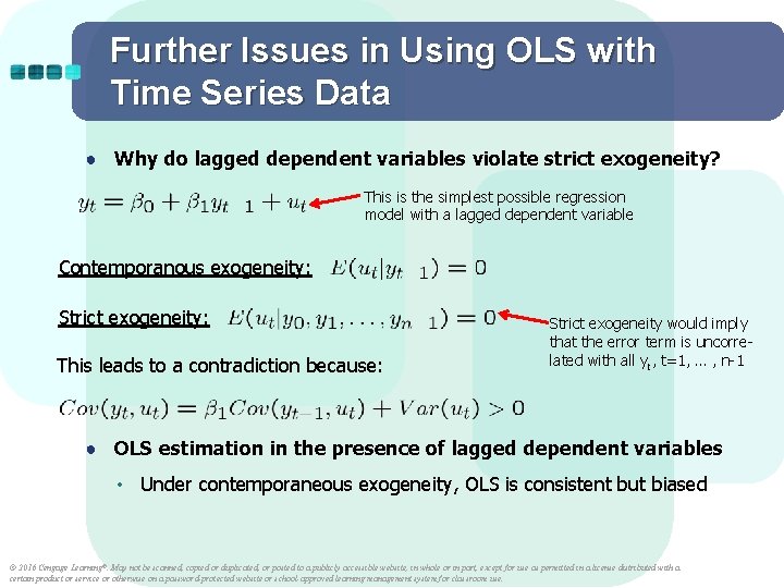
Further Issues in Using OLS with Time Series Data ● Why do lagged dependent variables violate strict exogeneity? This is the simplest possible regression model with a lagged dependent variable Contemporanous exogeneity: Strict exogeneity: This leads to a contradiction because: Strict exogeneity would imply that the error term is uncorrelated with all yt, t=1, … , n-1 ● OLS estimation in the presence of lagged dependent variables • Under contemporaneous exogeneity, OLS is consistent but biased © 2016 Cengage Learning®. May not be scanned, copied or duplicated, or posted to a publicly accessible website, in whole or in part, except for use as permitted in a license distributed with a certain product or service or otherwise on a password-protected website or school-approved learning management system for classroom use.

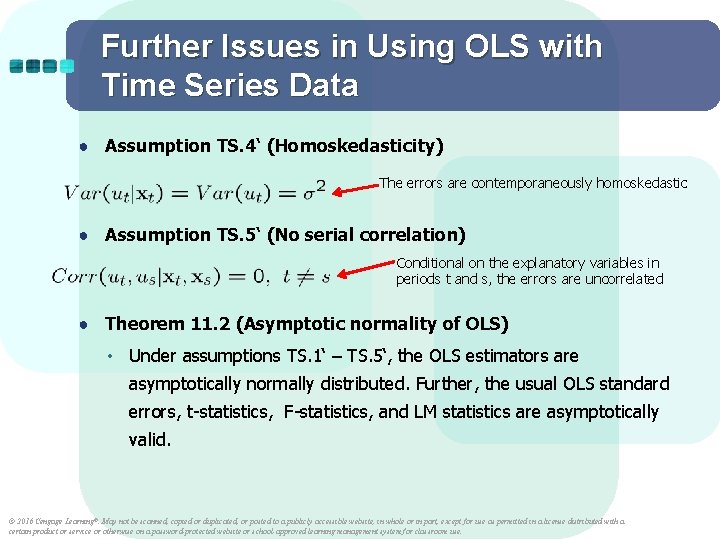
Further Issues in Using OLS with Time Series Data ● Assumption TS. 4‘ (Homoskedasticity) The errors are contemporaneously homoskedastic ● Assumption TS. 5‘ (No serial correlation) Conditional on the explanatory variables in periods t and s, the errors are uncorrelated ● Theorem 11. 2 (Asymptotic normality of OLS) • Under assumptions TS. 1‘ – TS. 5‘, the OLS estimators are asymptotically normally distributed. Further, the usual OLS standard errors, t-statistics, F-statistics, and LM statistics are asymptotically valid. © 2016 Cengage Learning®. May not be scanned, copied or duplicated, or posted to a publicly accessible website, in whole or in part, except for use as permitted in a license distributed with a certain product or service or otherwise on a password-protected website or school-approved learning management system for classroom use.

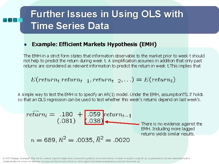
Further Issues in Using OLS with Time Series Data ● Example: Efficient Markets Hypothesis (EMH) The EMH in a strict form states that information observable to the market prior to week t should not help to predict the return during week t. A simplification assumes in addition that only past returns are considered as relevant information to predict the return in week t. This implies that A simple way to test the EMH is to specify an AR(1) model. Under the EMH, assumption. TS. 3‘ holds so that an OLS regression can be used to test whether this week‘s returns depend on last week‘s. There is no evidence against the EMH. Including more lagged returns yields similar results. © 2016 Cengage Learning®. May not be scanned, copied or duplicated, or posted to a publicly accessible website, in whole or in part, except for use as permitted in a license distributed with a certain product or service or otherwise on a password-protected website or school-approved learning management system for classroom use.

Further Issues in Using OLS with Time Series Data ● Using trend-stationary series in regression analysis • Time series with deterministic time trends are nonstationary • If they are stationary around the trend and in addition weakly dependent, they are called trend-stationary processes • Trend-stationary processes also satisfy assumption TS. 1‘ ● Using highly persistent time series in regression analysis • Unfortunately many economic time series violate weak dependence because they are highly persistent (= strongly dependent) • In this case OLS methods are generally invalid (unless the CLM hold) • In some cases transformations to weak dependence are possible © 2016 Cengage Learning®. May not be scanned, copied or duplicated, or posted to a publicly accessible website, in whole or in part, except for use as permitted in a license distributed with a certain product or service or otherwise on a password-protected website or school-approved learning management system for classroom use.

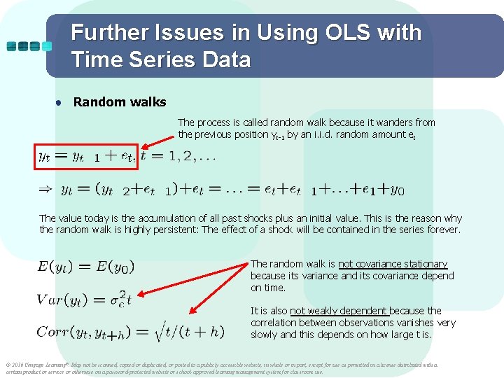
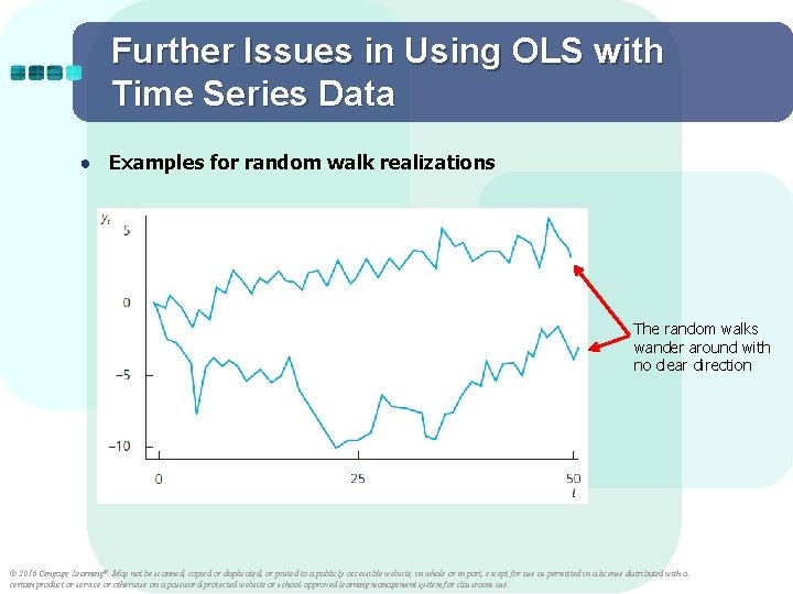
Further Issues in Using OLS with Time Series Data ● Random walks The process is called random walk because it wanders from the previous position yt-1 by an i. i. d. random amount et The value today is the accumulation of all past shocks plus an initial value. This is the reason why the random walk is highly persistent: The effect of a shock will be contained in the series forever. The random walk is not covariance stationary because its variance and its covariance depend on time. It is also not weakly dependent because the correlation between observations vanishes very slowly and this depends on how large t is. © 2016 Cengage Learning®. May not be scanned, copied or duplicated, or posted to a publicly accessible website, in whole or in part, except for use as permitted in a license distributed with a certain product or service or otherwise on a password-protected website or school-approved learning management system for classroom use.

Further Issues in Using OLS with Time Series Data ● Examples for random walk realizations The random walks wander around with no clear direction © 2016 Cengage Learning®. May not be scanned, copied or duplicated, or posted to a publicly accessible website, in whole or in part, except for use as permitted in a license distributed with a certain product or service or otherwise on a password-protected website or school-approved learning management system for classroom use.

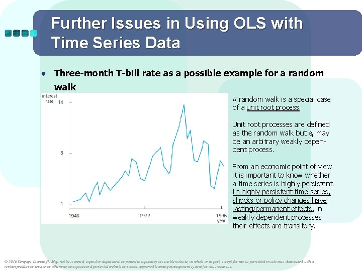
Further Issues in Using OLS with Time Series Data ● Three-month T-bill rate as a possible example for a random walk A random walk is a special case of a unit root process. Unit root processes are defined as the random walk but et may be an arbitrary weakly dependent process. From an economic point of view it is important to know whether a time series is highly persistent. In highly persistent time series, shocks or policy changes have lasting/permanent effects, in weakly dependent processes their effects are transitory. © 2016 Cengage Learning®. May not be scanned, copied or duplicated, or posted to a publicly accessible website, in whole or in part, except for use as permitted in a license distributed with a certain product or service or otherwise on a password-protected website or school-approved learning management system for classroom use.

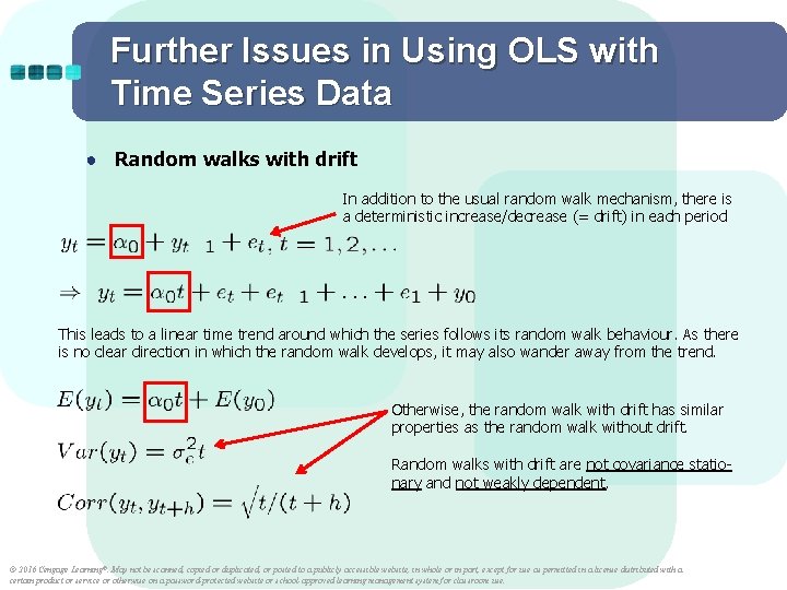
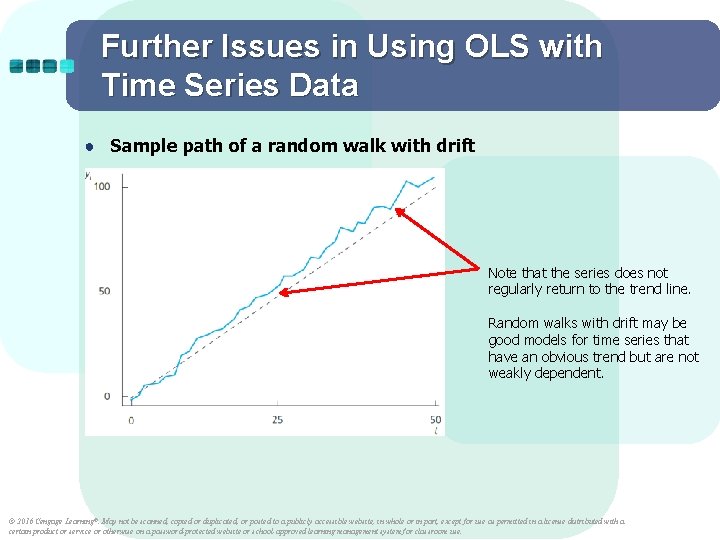
Further Issues in Using OLS with Time Series Data ● Random walks with drift In addition to the usual random walk mechanism, there is a deterministic increase/decrease (= drift) in each period This leads to a linear time trend around which the series follows its random walk behaviour. As there is no clear direction in which the random walk develops, it may also wander away from the trend. Otherwise, the random walk with drift has similar properties as the random walk without drift. Random walks with drift are not covariance stationary and not weakly dependent. © 2016 Cengage Learning®. May not be scanned, copied or duplicated, or posted to a publicly accessible website, in whole or in part, except for use as permitted in a license distributed with a certain product or service or otherwise on a password-protected website or school-approved learning management system for classroom use.

Further Issues in Using OLS with Time Series Data ● Sample path of a random walk with drift Note that the series does not regularly return to the trend line. Random walks with drift may be good models for time series that have an obvious trend but are not weakly dependent. © 2016 Cengage Learning®. May not be scanned, copied or duplicated, or posted to a publicly accessible website, in whole or in part, except for use as permitted in a license distributed with a certain product or service or otherwise on a password-protected website or school-approved learning management system for classroom use.

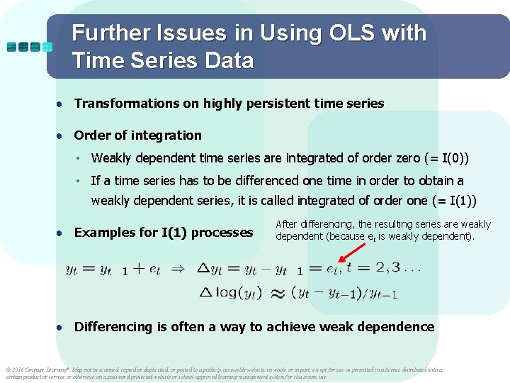
Further Issues in Using OLS with Time Series Data ● Transformations on highly persistent time series ● Order of integration • Weakly dependent time series are integrated of order zero (= I(0)) • If a time series has to be differenced one time in order to obtain a weakly dependent series, it is called integrated of order one (= I(1)) ● Examples for I(1) processes After differencing, the resulting series are weakly dependent (because et is weakly dependent). ● Differencing is often a way to achieve weak dependence © 2016 Cengage Learning®. May not be scanned, copied or duplicated, or posted to a publicly accessible website, in whole or in part, except for use as permitted in a license distributed with a certain product or service or otherwise on a password-protected website or school-approved learning management system for classroom use.

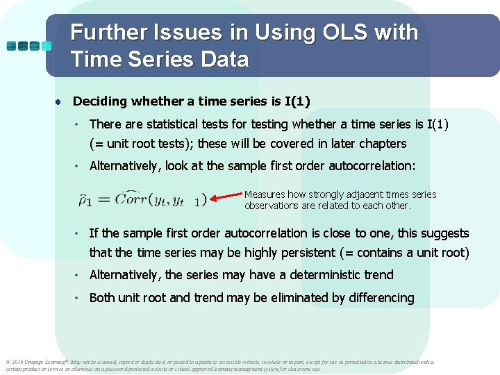
Further Issues in Using OLS with Time Series Data ● Deciding whether a time series is I(1) • There are statistical tests for testing whether a time series is I(1) (= unit root tests); these will be covered in later chapters • Alternatively, look at the sample first order autocorrelation: Measures how strongly adjacent times series observations are related to each other. • If the sample first order autocorrelation is close to one, this suggests that the time series may be highly persistent (= contains a unit root) • Alternatively, the series may have a deterministic trend • Both unit root and trend may be eliminated by differencing © 2016 Cengage Learning®. May not be scanned, copied or duplicated, or posted to a publicly accessible website, in whole or in part, except for use as permitted in a license distributed with a certain product or service or otherwise on a password-protected website or school-approved learning management system for classroom use.

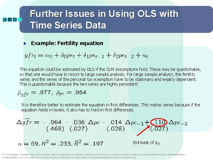
Further Issues in Using OLS with Time Series Data ● Example: Fertility equation This equation could be estimated by OLS if the CLM assumptions hold. These may be questionable, so that one would have to resort to large sample analysis. For large sample analysis, the fertility series and the series of the personal tax exemption have to be stationary and weakly dependent. This is • questionable because the two series are highly persistent: It is therefore better to estimate the equation in first differences. This makes sense because if the equation holds in levels, it also has to hold in first differences: Estimate of © 2016 Cengage Learning®. May not be scanned, copied or duplicated, or posted to a publicly accessible website, in whole or in part, except for use as permitted in a license distributed with a certain product or service or otherwise on a password-protected website or school-approved learning management system for classroom use.

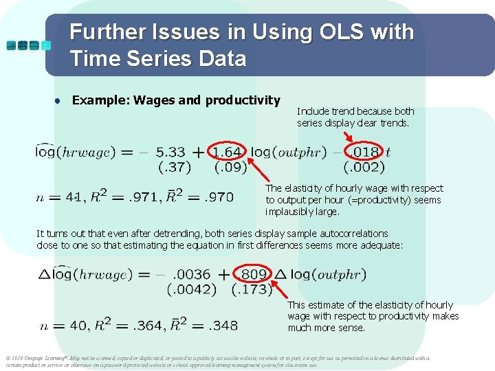
Further Issues in Using OLS with Time Series Data ● Example: Wages and productivity • Include trend because both series display clear trends. The elasticity of hourly wage with respect to output per hour (=productivity) seems implausibly large. It turns out that even after detrending, both series display sample autocorrelations close to one so that estimating the equation in first differences seems more adequate: This estimate of the elasticity of hourly wage with respect to productivity makes much more sense. © 2016 Cengage Learning®. May not be scanned, copied or duplicated, or posted to a publicly accessible website, in whole or in part, except for use as permitted in a license distributed with a certain product or service or otherwise on a password-protected website or school-approved learning management system for classroom use.

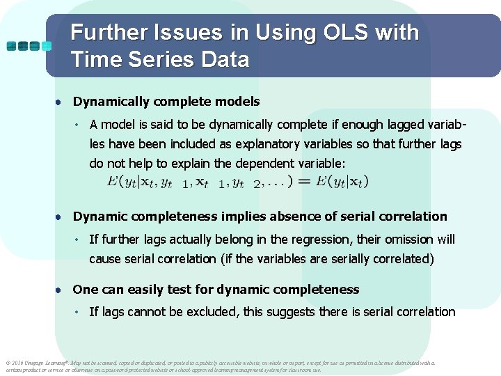
Further Issues in Using OLS with Time Series Data ● Dynamically complete models • A model is said to be dynamically complete if enough lagged variables have been included as explanatory variables so that further lags do not help to explain the dependent variable: ● Dynamic completeness implies absence of serial correlation • If further lags actually belong in the regression, their omission will cause serial correlation (if the variables are serially correlated) ● One can easily test for dynamic completeness • If lags cannot be excluded, this suggests there is serial correlation © 2016 Cengage Learning®. May not be scanned, copied or duplicated, or posted to a publicly accessible website, in whole or in part, except for use as permitted in a license distributed with a certain product or service or otherwise on a password-protected website or school-approved learning management system for classroom use.

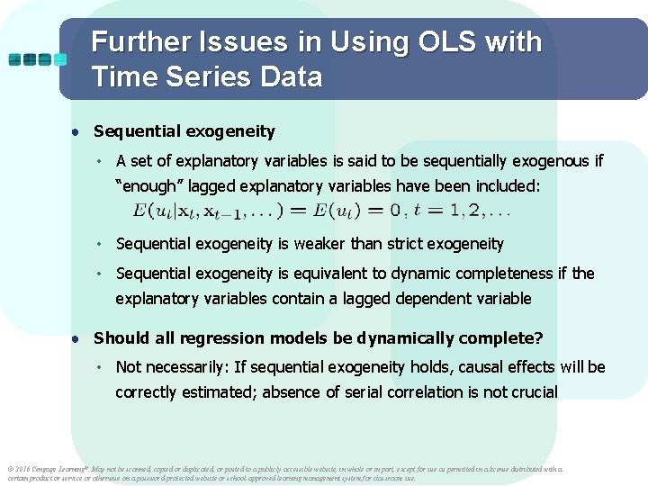
Further Issues in Using OLS with Time Series Data ● Sequential exogeneity • A set of explanatory variables is said to be sequentially exogenous if “enough” lagged explanatory variables have been included: • Sequential exogeneity is weaker than strict exogeneity • Sequential exogeneity is equivalent to dynamic completeness if the explanatory variables contain a lagged dependent variable ● Should all regression models be dynamically complete? • Not necessarily: If sequential exogeneity holds, causal effects will be correctly estimated; absence of serial correlation is not crucial © 2016 Cengage Learning®. May not be scanned, copied or duplicated, or posted to a publicly accessible website, in whole or in part, except for use as permitted in a license distributed with a certain product or service or otherwise on a password-protected website or school-approved learning management system for classroom use.