Chapter 10 Correlation and Regression 10 2 Correlation

Chapter 10 Correlation and Regression 10 -2 Correlation 10 -3 Regression Copyright © 2014, 2012, 2010 Pearson Education, Inc. Section 10. 2 -1

Key Concept Part 1 of this section introduces the linear correlation coefficient, r, which is a number that measures how well paired sample data fit a straight-line pattern when graphed. Using paired sample data (sometimes called bivariate data), we find the value of r (usually using technology), then we use that value to conclude that there is (or is not) a linear correlation between the two variables. In this section we consider only linear relationships, which means that when graphed, the points approximate a straight-line pattern. Copyright © 2014, 2012, 2010 Pearson Education, Inc. Section 10. 2 -2

Definition A correlation exists between two variables when the values of one are somehow associated with the values of the other in some way. A linear correlation exists between two variables when there is a correlation and the plotted points of paired data result in a pattern that can be approximated by a straight line. Copyright © 2014, 2012, 2010 Pearson Education, Inc. Section 10. 2 -3

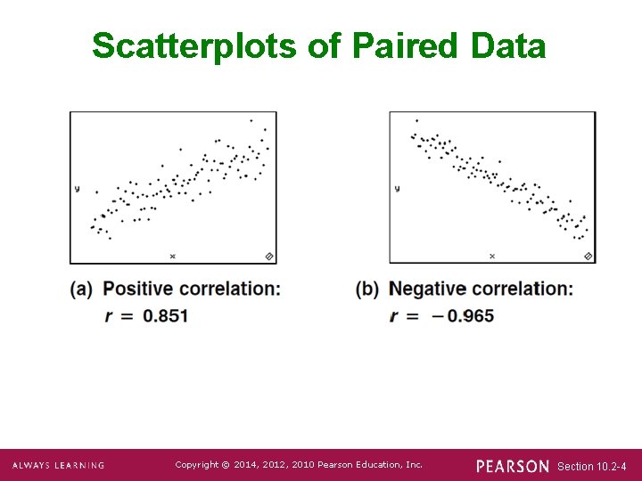
Scatterplots of Paired Data Copyright © 2014, 2012, 2010 Pearson Education, Inc. Section 10. 2 -4

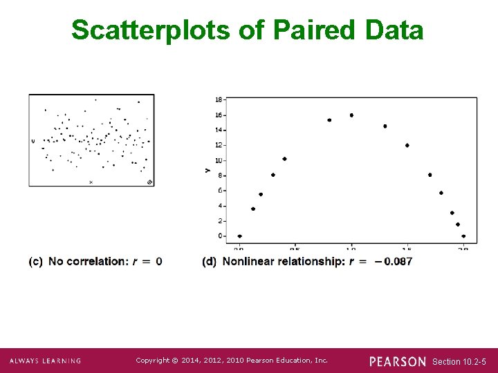
Scatterplots of Paired Data Copyright © 2014, 2012, 2010 Pearson Education, Inc. Section 10. 2 -5

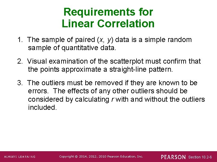
Requirements for Linear Correlation 1. The sample of paired (x, y) data is a simple random sample of quantitative data. 2. Visual examination of the scatterplot must confirm that the points approximate a straight-line pattern. 3. The outliers must be removed if they are known to be errors. The effects of any other outliers should be considered by calculating r with and without the outliers included. Copyright © 2014, 2012, 2010 Pearson Education, Inc. Section 10. 2 -6

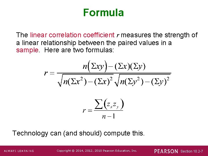
Formula The linear correlation coefficient r measures the strength of a linear relationship between the paired values in a sample. Here are two formulas: Technology can (and should) compute this. Copyright © 2014, 2012, 2010 Pearson Education, Inc. Section 10. 2 -7

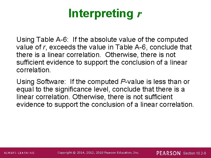
Interpreting r Using Table A-6: If the absolute value of the computed value of r, exceeds the value in Table A-6, conclude that there is a linear correlation. Otherwise, there is not sufficient evidence to support the conclusion of a linear correlation. Using Software: If the computed P-value is less than or equal to the significance level, conclude that there is a linear correlation. Otherwise, there is not sufficient evidence to support the conclusion of a linear correlation. Copyright © 2014, 2012, 2010 Pearson Education, Inc. Section 10. 2 -8

Caution Know that the methods of this section apply to a linear correlation. If you conclude that there does not appear to be linear correlation, know that it is possible that there might be some other association that is not linear. Copyright © 2014, 2012, 2010 Pearson Education, Inc. Section 10. 2 -9

Properties of the Linear Correlation Coefficient r 1. – 1 ≤ r ≤ 1 2. If all values of either variable are converted to a different scale, the value of r does not change. 3. The value of r is not affected by the choice of x and y. Interchange all x- and y-values and the value of r will not change. 4. r measures strength of a linear relationship. 5. r is very sensitive to outliers, which can dramatically affect the value of r. Copyright © 2014, 2012, 2010 Pearson Education, Inc. Section 10. 2 -10

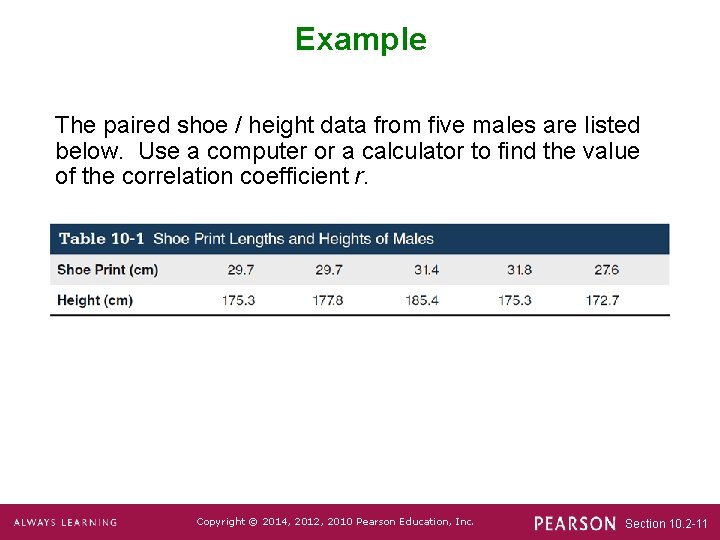
Example The paired shoe / height data from five males are listed below. Use a computer or a calculator to find the value of the correlation coefficient r. Copyright © 2014, 2012, 2010 Pearson Education, Inc. Section 10. 2 -11

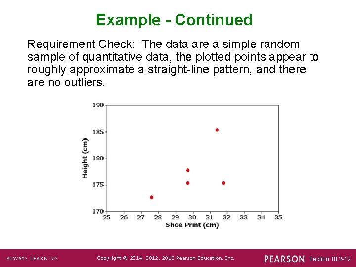
Example - Continued Requirement Check: The data are a simple random sample of quantitative data, the plotted points appear to roughly approximate a straight-line pattern, and there are no outliers. Copyright © 2014, 2012, 2010 Pearson Education, Inc. Section 10. 2 -12

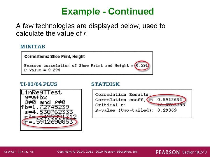
Example - Continued A few technologies are displayed below, used to calculate the value of r. Copyright © 2014, 2012, 2010 Pearson Education, Inc. Section 10. 2 -13

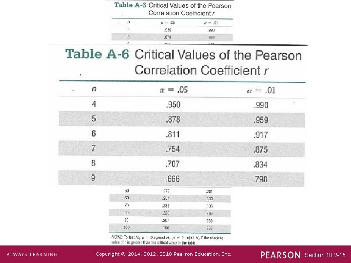
Is There a Linear Correlation? We found previously for the shoe and height example that r = 0. 591. We now proceed to interpret its meaning. Our goal is to decide whether or not there appears to be a linear correlation between shoe print lengths and heights of people. We can base our interpretation on a critical value from Table A-6. Copyright © 2014, 2012, 2010 Pearson Education, Inc. Section 10. 2 -14

Copyright © 2014, 2012, 2010 Pearson Education, Inc. Section 10. 2 -15

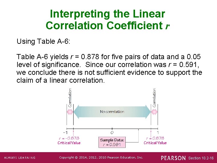
Interpreting the Linear Correlation Coefficient r Using Table A-6: Table A-6 yields r = 0. 878 for five pairs of data and a 0. 05 level of significance. Since our correlation was r = 0. 591, we conclude there is not sufficient evidence to support the claim of a linear correlation. Copyright © 2014, 2012, 2010 Pearson Education, Inc. Section 10. 2 -16

Interpreting r: Explained Variation The value of r 2 is the proportion of the variation in y that is explained by the linear relationship between x and y. Copyright © 2014, 2012, 2010 Pearson Education, Inc. Section 10. 2 -17

Example We found previously for the shoe and height example that r = 0. 591. With r = 0. 591, we get r 2 = 0. 349. We conclude that about 34. 9% of the variation in height can be explained by the linear relationship between lengths of shoe prints and heights. Copyright © 2014, 2012, 2010 Pearson Education, Inc. Section 10. 2 -18

Caution Know that correlation does not imply causality. Copyright © 2014, 2012, 2010 Pearson Education, Inc. Section 10. 2 -19

Chapter 10 Correlation and Regression 10 -2 Correlation 10 -3 Regression Copyright © 2014, 2012, 2010 Pearson Education, Inc. Section 10. 2 -20

Key Concept In Part 1 of this section we find the equation of the straight line that best fits the paired sample data. That equation algebraically describes the relationship between two variables. The best-fitting straight line is called a regression line and its equation is called the regression equation. Copyright © 2014, 2012, 2010 Pearson Education, Inc. Section 10. 2 -21

Definitions Regression Equation: Given a collection of paired sample data, the regression line (or line of best fit, or least-squares line) is the straight line that “best” fits the scatterplot of data. The regression equation ŷ = b 0 + b 1 x algebraically describes the regression line. Copyright © 2014, 2012, 2010 Pearson Education, Inc. Section 10. 2 -22

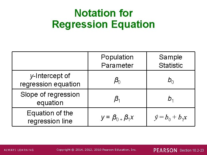
Notation for Regression Equation Population Parameter Sample Statistic y-Intercept of regression equation β 0 b 0 Slope of regression equation β 1 b 1 Equation of the regression line y = β 0 + β 1 x ŷ = b 0 + b 1 x Copyright © 2014, 2012, 2010 Pearson Education, Inc. Section 10. 2 -23

Requirements 1. The sample of paired (x, y) data is a random sample of quantitative data. 2. Visual examination of the scatterplot shows that the points approximate a straight-line pattern. 3. Any outliers must be removed if they are known to be errors. Consider the effects of any outliers that are not known errors. Copyright © 2014, 2012, 2010 Pearson Education, Inc. Section 10. 2 -24

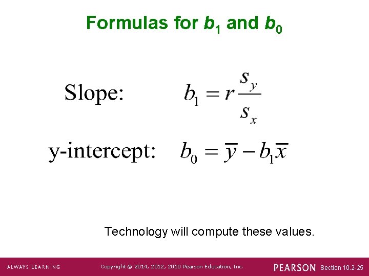
Formulas for b 1 and b 0 Technology will compute these values. Copyright © 2014, 2012, 2010 Pearson Education, Inc. Section 10. 2 -25

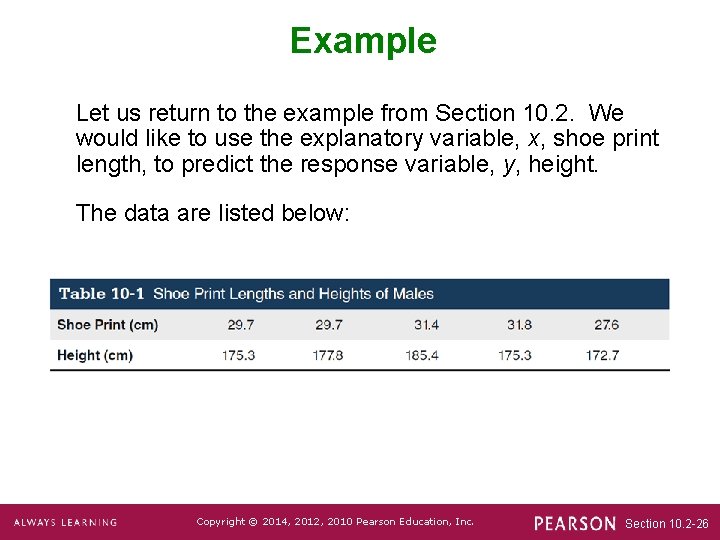
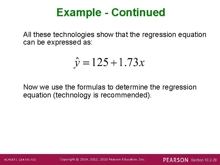
Example Let us return to the example from Section 10. 2. We would like to use the explanatory variable, x, shoe print length, to predict the response variable, y, height. The data are listed below: Copyright © 2014, 2012, 2010 Pearson Education, Inc. Section 10. 2 -26

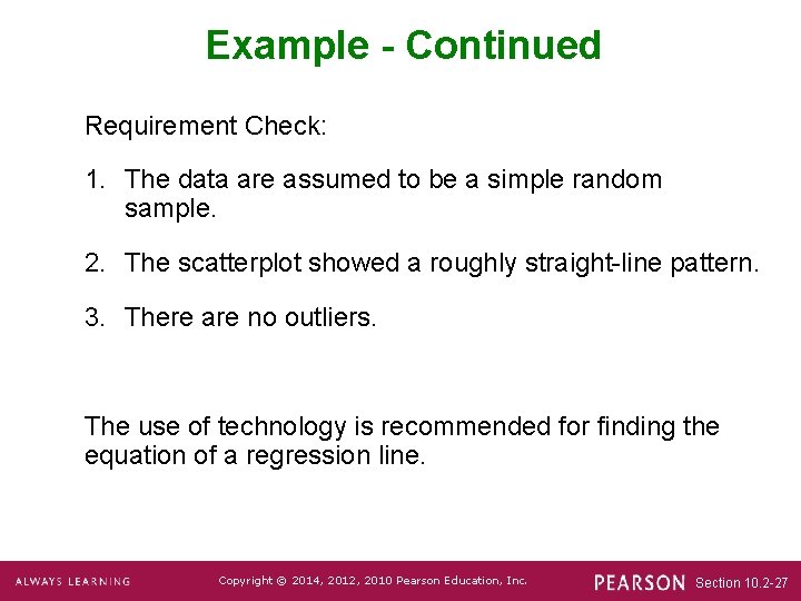
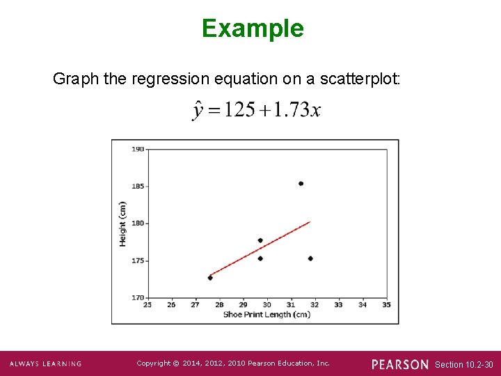
Example - Continued Requirement Check: 1. The data are assumed to be a simple random sample. 2. The scatterplot showed a roughly straight-line pattern. 3. There are no outliers. The use of technology is recommended for finding the equation of a regression line. Copyright © 2014, 2012, 2010 Pearson Education, Inc. Section 10. 2 -27

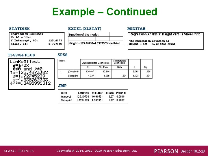
Example – Continued Copyright © 2014, 2012, 2010 Pearson Education, Inc. Section 10. 2 -28

Example - Continued All these technologies show that the regression equation can be expressed as: Now we use the formulas to determine the regression equation (technology is recommended). Copyright © 2014, 2012, 2010 Pearson Education, Inc. Section 10. 2 -29

Example Graph the regression equation on a scatterplot: Copyright © 2014, 2012, 2010 Pearson Education, Inc. Section 10. 2 -30

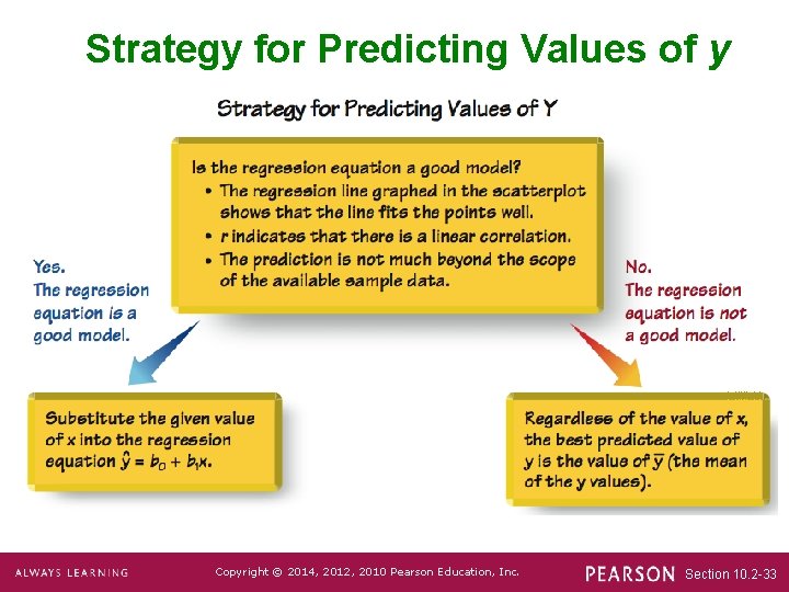
Using the Regression Equation for Predictions 1. Use the regression equation for predictions only if the graph of the regression line on the scatterplot confirms that the regression line fits the points reasonably well. 2. Use the regression equation for predictions only if the linear correlation coefficient r indicates that there is a linear correlation between the two variables (as described in Section 10 -2). Copyright © 2014, 2012, 2010 Pearson Education, Inc. Section 10. 2 -31

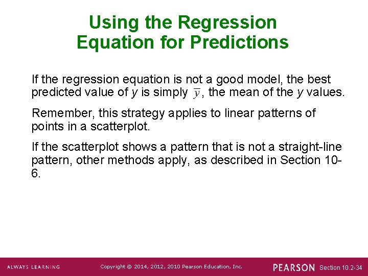
Using the Regression Equation for Predictions 3. Use the regression line for predictions only if the data do not go much beyond the scope of the available sample data. (Predicting too far beyond the scope of the available sample data is called extrapolation, and it could result in bad predictions. ) 4. If the regression equation does not appear to be useful for making predictions, the best predicted value of a variable is its sample mean. Copyright © 2014, 2012, 2010 Pearson Education, Inc. Section 10. 2 -32

Strategy for Predicting Values of y Copyright © 2014, 2012, 2010 Pearson Education, Inc. Section 10. 2 -33

Using the Regression Equation for Predictions If the regression equation is not a good model, the best predicted value of y is simply , the mean of the y values. Remember, this strategy applies to linear patterns of points in a scatterplot. If the scatterplot shows a pattern that is not a straight-line pattern, other methods apply, as described in Section 106. Copyright © 2014, 2012, 2010 Pearson Education, Inc. Section 10. 2 -34

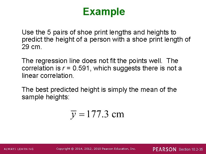
Example Use the 5 pairs of shoe print lengths and heights to predict the height of a person with a shoe print length of 29 cm. The regression line does not fit the points well. The correlation is r = 0. 591, which suggests there is not a linear correlation. The best predicted height is simply the mean of the sample heights: Copyright © 2014, 2012, 2010 Pearson Education, Inc. Section 10. 2 -35

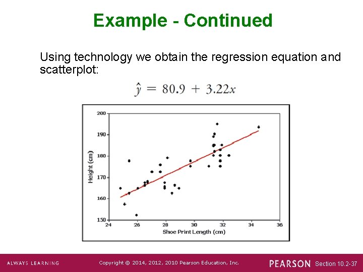
Example Use the 40 pairs of shoe print lengths from Data Set 2 in Appendix B to predict the height of a person with a shoe print length of 29 cm. Now, the regression line does fit the points well, and the correlation of r = 0. 813 suggests that there is a linear correlation. Copyright © 2014, 2012, 2010 Pearson Education, Inc. Section 10. 2 -36

Example - Continued Using technology we obtain the regression equation and scatterplot: Copyright © 2014, 2012, 2010 Pearson Education, Inc. Section 10. 2 -37

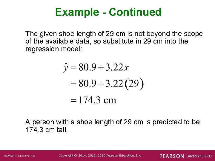
Example - Continued The given shoe length of 29 cm is not beyond the scope of the available data, so substitute in 29 cm into the regression model: A person with a shoe length of 29 cm is predicted to be 174. 3 cm tall. Copyright © 2014, 2012, 2010 Pearson Education, Inc. Section 10. 2 -38