Graph Theory Chapter 2 Trees and Distance 2

Graph Theory Chapter 2 Trees and Distance 2. 1 Basic properties 2. 2 Spanning tree and enumeration 2. 3 Optimization and trees Ch. 2. Trees and Distance 1

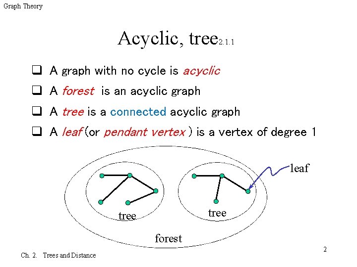
Graph Theory Acyclic, tree 2. 1. 1 q A graph with no cycle is acyclic q A forest is an acyclic graph q A tree is a connected acyclic graph q A leaf (or pendant vertex ) is a vertex of degree 1 leaf tree forest Ch. 2. Trees and Distance 2

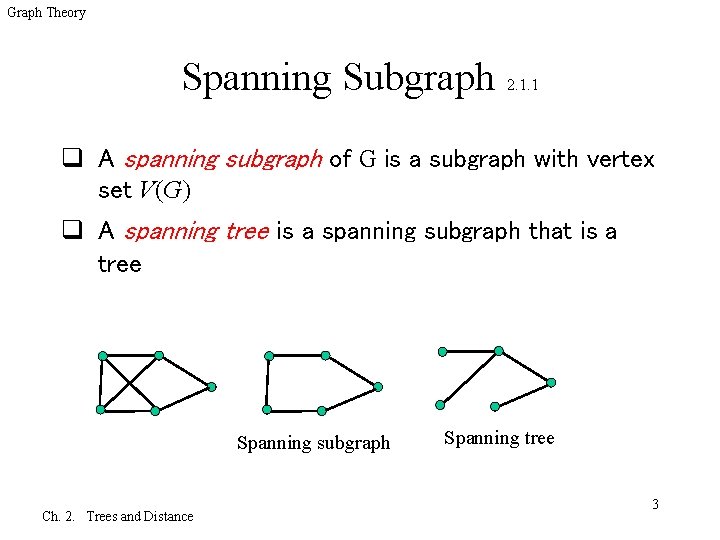
Graph Theory Spanning Subgraph 2. 1. 1 q A spanning subgraph of G is a subgraph with vertex set V(G) q A spanning tree is a spanning subgraph that is a tree Spanning subgraph Ch. 2. Trees and Distance Spanning tree 3

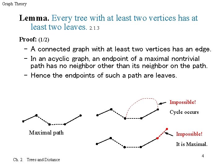
Graph Theory Lemma. Every tree with at least two vertices has at least two leaves. 2. 1. 3 Proof: (1/2) – A connected graph with at least two vertices has an edge. – In an acyclic graph, an endpoint of a maximal nontrivial path has no neighbor other than its neighbor on the path. – Hence the endpoints of such a path are leaves. Impossible! Cycle occurs Maximal path Impossible! It is Maximal. Ch. 2. Trees and Distance 4

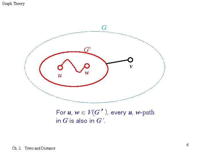
Graph Theory Lemma. Deleting a leaf from a n-vertex tree produces a tree with n-1 vertices. 2. 1. 3 Proof: (2/2) – Let v be a leaf of a tree G, and that G’=G-v. – A vertex of degree 1 belongs to no path connecting two other vertices. – Therefore, for u, w V(G’), every u, w-path in G is also in G’. – Hence G’ is connected. – Since deleting a vertex cannot create a cycle, G’ also is acyclic. – Thus G’ is a tree with n-1 vertices. Ch. 2. Trees and Distance 5

Graph Theory G G’ u w v For u, w V(G’ ), every u, w-path in G is also in G’. Ch. 2. Trees and Distance 6

Graph Theory Theorem 2. 1. 4. For an n-vertex graph G (with n 1), the following are equivalent (and characterize the trees with n vertices) 2. 1. 4 A) G is connected and has no cycles B) G is connected and has n-1 edges C) G has n-1 edges and no cycles D) For u, v V(G), G has exactly one u, v-path Proof: We first demonstrate the equivalence of A, B, and C by proving that any two of {connected, acyclic, n-1 edges} together imply the third Ch. 2. Trees and Distance 7

Graph Theory A {B, C}. connected, acyclic n-1 edges Theorem 2. 1. 4 Continue q We use induction on n. q For n=1, an acyclic 1 -vertex graph has no edge q For n >1, we suppose that implication holds for graphs with fewer than n vertices – Given an acyclic connected graph G, Lemma 2. 1. 3 provides a leaf v and states that G’=G-v also is acyclic and connected (see figure in previous proof) – Applying the induction hypothesis to G’ yields e(G’)=n-2 – Since only one edge is incident to v, we have e(G)=n-1 Ch. 2. Trees and Distance 8

Graph Theory B {A, C} Connected and n-1 edges acyclic Theorem 2. 1. 4 continue q If G is not acyclic, delete edges from cycles of G one by one until the resulting graph G’ is acyclic q Since no edge of a cycle is a cut-edge(Theorem 1. 2. 14), G’ is connected – Now the preceding paragraph implies that = n-1 e(G’) – Since we are given e(G)=n-1, no edges were deleted q Thus G’=G, and G is acyclic Ch. 2. Trees and Distance 9

Graph Theory C {A, B} n-1 edges and no cycles connected Theorem 2. 1. 4 continue q Let G 1, …, Gk be the components of G q Since every vertex appears in one component, in(Gi)=n – Since G has no cycles, each component satisfies property A. Thus e(Gi) = n(Gi) - 1 – Summing over i yields e(G)= I[n(Gi)-1]= n-k q We are given e(G)=n-1, so k =1, and G is connected Ch. 2. Trees and Distance 10

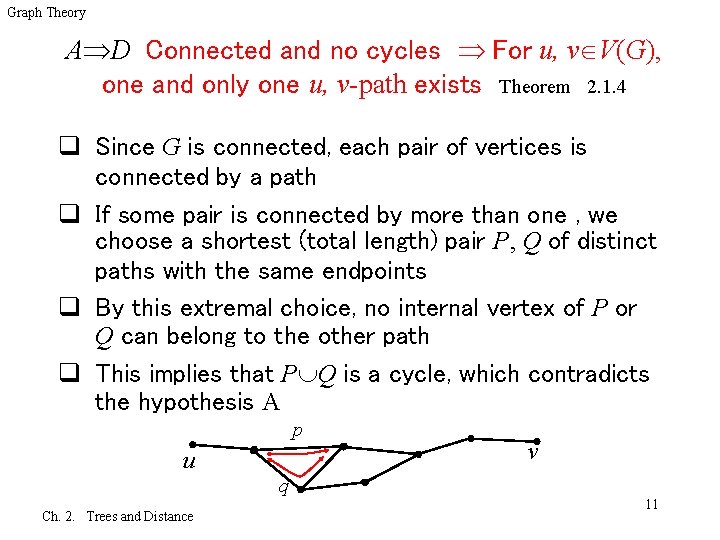
Graph Theory A D Connected and no cycles For u, v V(G), one and only one u, v-path exists Theorem 2. 1. 4 q Since G is connected, each pair of vertices is connected by a path q If some pair is connected by more than one , we choose a shortest (total length) pair P, Q of distinct paths with the same endpoints q By this extremal choice, no internal vertex of P or Q can belong to the other path q This implies that P Q is a cycle, which contradicts the hypothesis A p u v q Ch. 2. Trees and Distance 11

Graph Theory D A For u, v V(G), one and only one u, v-path exists connected and no cycles Theorem 2. 1. 4 q If there is a u, v-path for every u, v V(G), then G is connected q If G has a cycle C, then G has two u, v-paths for u, v V(G); which contradicts the hypothesis D q Hence G is acyclic (this also forbids loops). Ch. 2. Trees and Distance 12

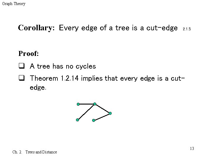
Graph Theory Corollary: Every edge of a tree is a cut-edge 2. 1. 5 Proof: q A tree has no cycles q Theorem 1. 2. 14 implies that every edge is a cutedge. Ch. 2. Trees and Distance 13

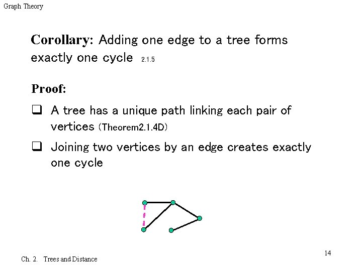
Graph Theory Corollary: Adding one edge to a tree forms exactly one cycle 2. 1. 5 Proof: q A tree has a unique path linking each pair of vertices (Theorem 2. 1. 4 D) q Joining two vertices by an edge creates exactly one cycle Ch. 2. Trees and Distance 14

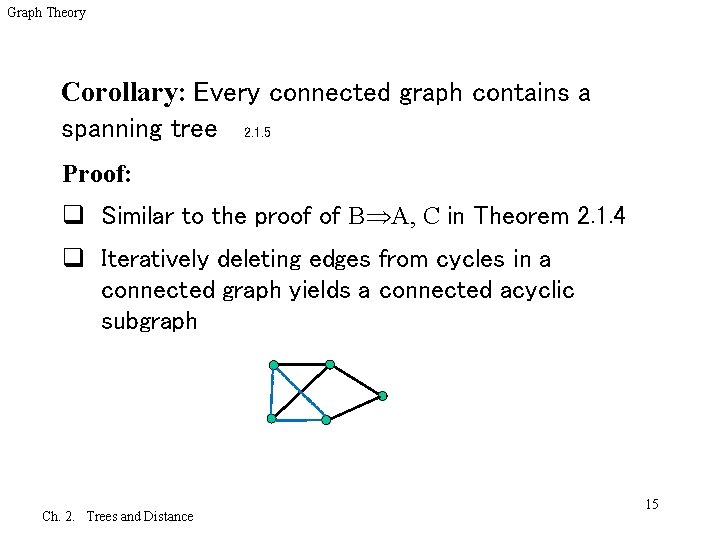
Graph Theory Corollary: Every connected graph contains a spanning tree 2. 1. 5 Proof: q Similar to the proof of B A, C in Theorem 2. 1. 4 q Iteratively deleting edges from cycles in a connected graph yields a connected acyclic subgraph Ch. 2. Trees and Distance 15

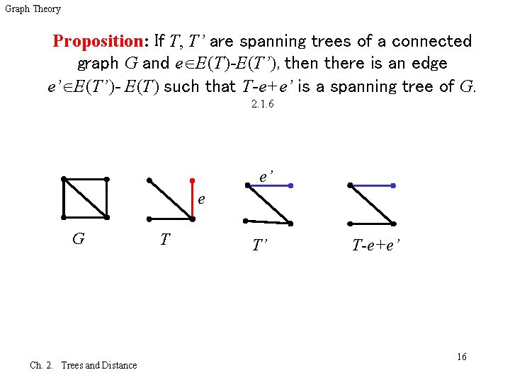
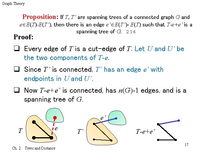
Graph Theory Proposition: If T, T’ are spanning trees of a connected graph G and e E(T)-E(T’), then there is an edge e’ E(T’)- E(T) such that T-e+e’ is a spanning tree of G. 2. 1. 6 e’ e G Ch. 2. Trees and Distance T T’ T-e+e’ 16

Graph Theory Proposition: If T, T’ are spanning trees of a connected graph G and e E(T)-E(T’), then there is an edge e’ E(T’)- E(T) such that T-e+e’ is a spanning tree of G. 2. 1. 6 Proof: q Every edge of T is a cut-edge of T. Let U and U’ be the two components of T-e. q Since T’ is connected, T’ has an edge e’ with endpoints in U and U’. q Now T-e+e’ is connected, has n(G)-1 edges, and is a spanning tree of G. e’ T e Ch. 2. Trees and Distance T’ T-e+e’ 17

Graph Theory Distance in trees and Graphs q Assume G has a u, v-path q Then the distance from u to v, written d. G(u, v) or d(u, v), is the least length of a u, v-path. q If G has no such path, then d(u, v)= Ch. 2. Trees and Distance 18

Graph Theory Distance in trees and Graphs q The diameter (diam G) is maxu, v V(G) d(u, v) – Upper bound of distance between every pair q The eccentricity of a vertex u is (u) = maxv V(G) d(u, v) – Upper bound of the distance from u to the others q The radius of a graph G is rad G = minu V(G) (u) – Lower bound of the eccentricity Ch. 2. Trees and Distance 19

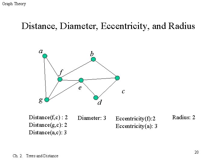
Graph Theory Distance, Diameter, Eccentricity, and Radius a b f e g Distance(f, c) : 2 Distance(g, c): 2 Distance(a, c): 3 Ch. 2. Trees and Distance c d Diameter: 3 Eccentricity(f): 2 Eccentricity(a): 3 Radius: 2 20

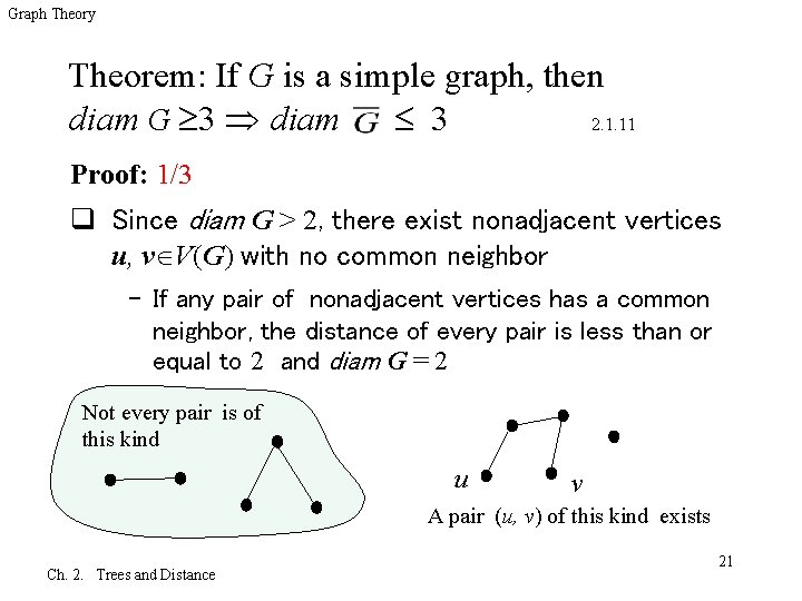
Graph Theory Theorem: If G is a simple graph, then diam G 3 diam 3 2. 1. 11 Proof: 1/3 q Since diam G > 2, there exist nonadjacent vertices u, v V(G) with no common neighbor – If any pair of nonadjacent vertices has a common neighbor, the distance of every pair is less than or equal to 2 and diam G = 2 Not every pair is of this kind u v A pair (u, v) of this kind exists Ch. 2. Trees and Distance 21

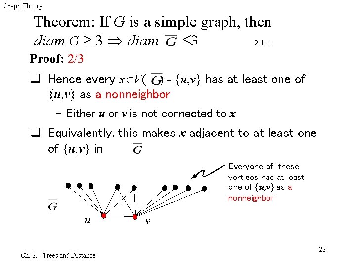
Graph Theory Theorem: If G is a simple graph, then diam G 3 diam 3 2. 1. 11 Proof: 2/3 q Hence every x V( ) - {u, v} has at least one of {u, v} as a nonneighbor – Either u or v is not connected to x q Equivalently, this makes x adjacent to at least one of {u, v} in Everyone of these vertices has at least one of {u, v} as a nonneighbor u Ch. 2. Trees and Distance v 22

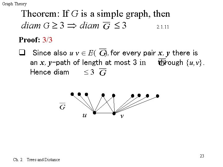
Graph Theory Theorem: If G is a simple graph, then diam G 3 diam 3 2. 1. 11 Proof: 3/3 q Since also u v E( ), for every pair x, y there is an x, y-path of length at most 3 in through {u, v}. Hence diam 3 u Ch. 2. Trees and Distance v 23

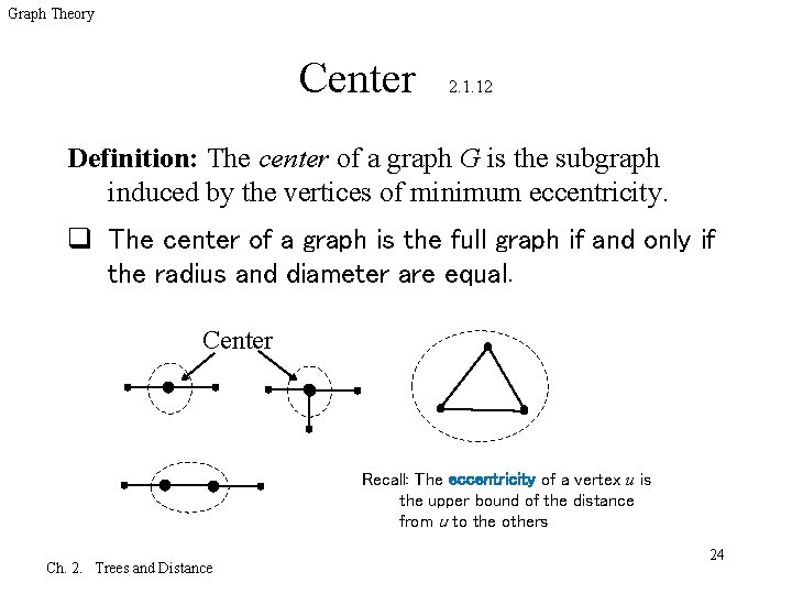
Graph Theory Center 2. 1. 12 Definition: The center of a graph G is the subgraph induced by the vertices of minimum eccentricity. q The center of a graph is the full graph if and only if the radius and diameter are equal. Center Recall: The eccentricity of a vertex u is the upper bound of the distance from u to the others Ch. 2. Trees and Distance 24

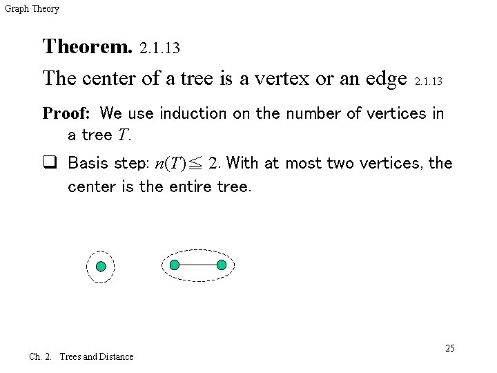
Graph Theory Theorem. 2. 1. 13 The center of a tree is a vertex or an edge 2. 1. 13 Proof: We use induction on the number of vertices in a tree T. q Basis step: n(T)≦ 2. With at most two vertices, the center is the entire tree. Ch. 2. Trees and Distance 25

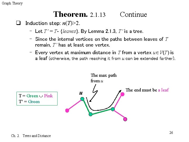
Graph Theory Theorem. 2. 1. 13 Continue q Induction step: n(T)>2. – Let T’ = T- {leaves}. By Lemma 2. 1. 3, T’ is a tree. – Since the internal vertices on the paths between leaves of T remain, T’ has at least one vertex. – Every vertex at maximum distance in T from a vertex u V(T) is a leaf (otherwise, the path reaching it from u can be extended farther). The max path from u T = Green Pink T’ = Green Ch. 2. Trees and Distance u The end must be a leaf 26

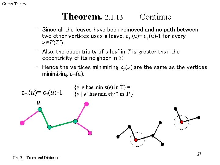
Graph Theory Theorem. 2. 1. 13 Continue – Since all the leaves have been removed and no path between two other vertices uses a leave, T’(u)= T(u)-1 for every u V(T’). – Also, the eccentricity of a leaf in T is greater than the eccentricity of its neighbor in T. – Hence the vertices minimizing T(u) are the same as the vertices minimizing T’(u)= T(u)-1 u Ch. 2. Trees and Distance {v| v has min (v) in T} = {v’| v’ has min (v’) in T’} 27

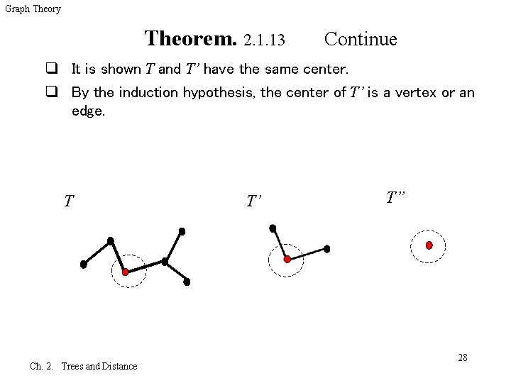
Graph Theory Theorem. 2. 1. 13 Continue q It is shown T and T’ have the same center. q By the induction hypothesis, the center of T’ is a vertex or an edge. T Ch. 2. Trees and Distance T’ T” 28

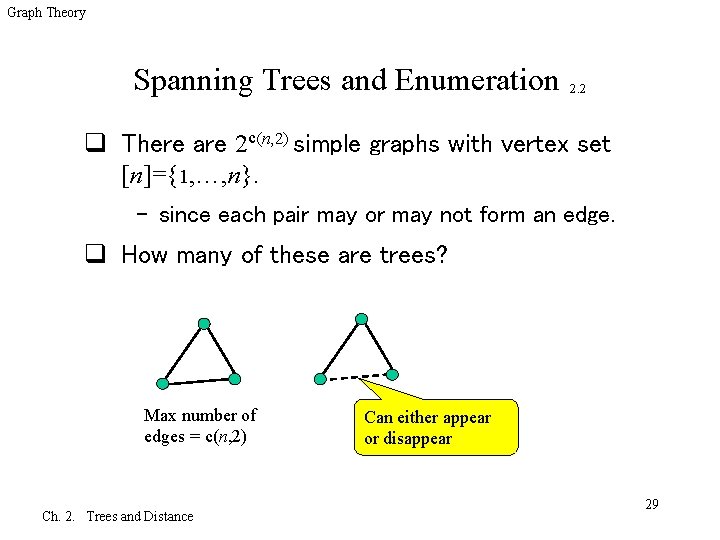
Graph Theory Spanning Trees and Enumeration 2. 2 q There are 2 c(n, 2) simple graphs with vertex set [n]={1, …, n}. – since each pair may or may not form an edge. q How many of these are trees? Max number of edges = c(n, 2) Ch. 2. Trees and Distance Can either appear or disappear 29

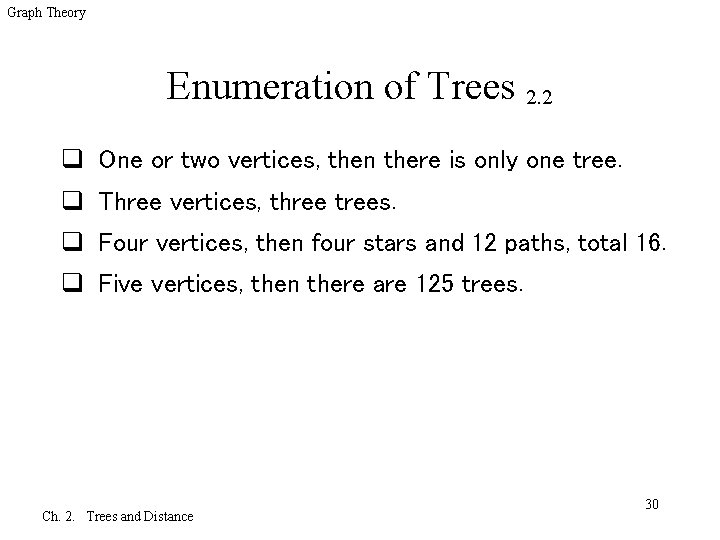
Graph Theory Enumeration of Trees 2. 2 q One or two vertices, then there is only one tree. q Three vertices, three trees. q Four vertices, then four stars and 12 paths, total 16. q Five vertices, then there are 125 trees. Ch. 2. Trees and Distance 30

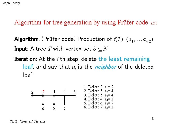
Graph Theory Algorithm for tree generation by using Prűfer code 2. 2. 1 Algorithm. (Prűfer code) Production of f(T)=(a 1, …, an-2) Input: A tree T with vertex set S N Iteration: At the i th step, delete the least remaining leaf, and say that ai is the neighbor of the deleted leaf 2 7 1 4 6 8 5 Ch. 2. Trees and Distance 3 1. Delete 2 2. Delete 3 3. Delete 5 4. Delete 4 5. Delete 6 6. Delete 7 a 1= 7 a 2= 4 a 3= 4 a 4= 1 a 5= 7 a 6= 1 31

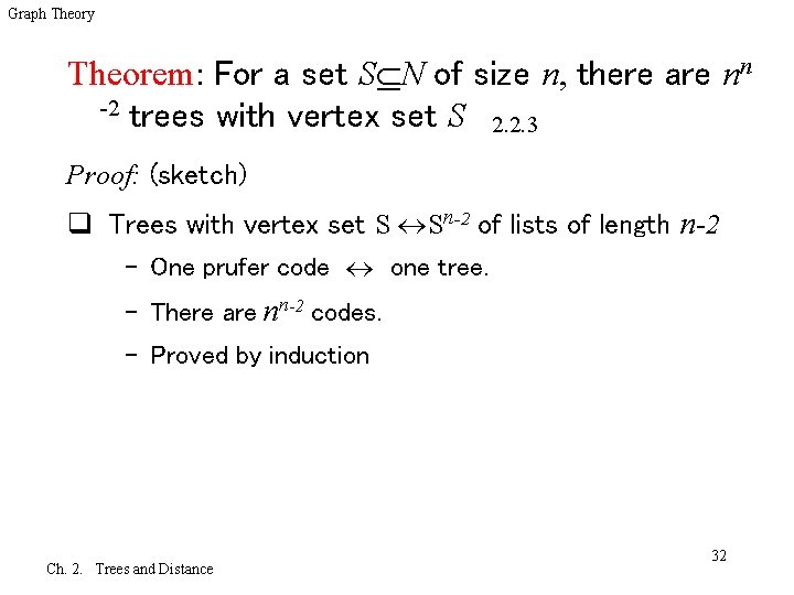
Graph Theory Theorem: For a set S N of size n, there are nn -2 trees with vertex set S 2. 2. 3 Proof: (sketch) q Trees with vertex set S Sn-2 of lists of length n-2 – One prufer code one tree. – There are nn-2 codes. – Proved by induction Ch. 2. Trees and Distance 32

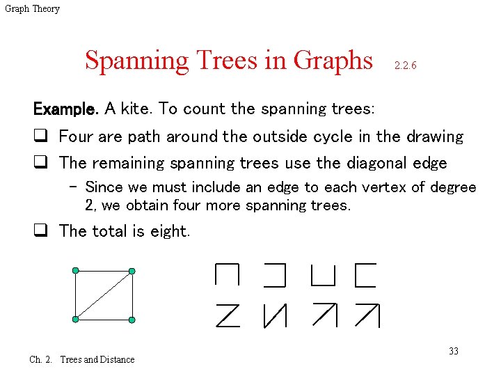
Graph Theory Spanning Trees in Graphs 2. 2. 6 Example. A kite. To count the spanning trees: q Four are path around the outside cycle in the drawing q The remaining spanning trees use the diagonal edge – Since we must include an edge to each vertex of degree 2, we obtain four more spanning trees. q The total is eight. Ch. 2. Trees and Distance 33

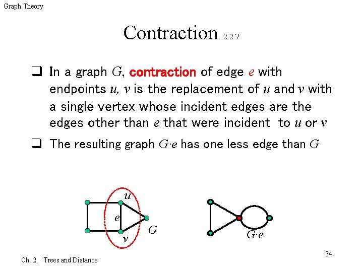
Graph Theory Contraction 2. 2. 7 q In a graph G, contraction of edge e with endpoints u, v is the replacement of u and v with a single vertex whose incident edges are the edges other than e that were incident to u or v q The resulting graph G·e has one less edge than G u e v Ch. 2. Trees and Distance G G·e 34

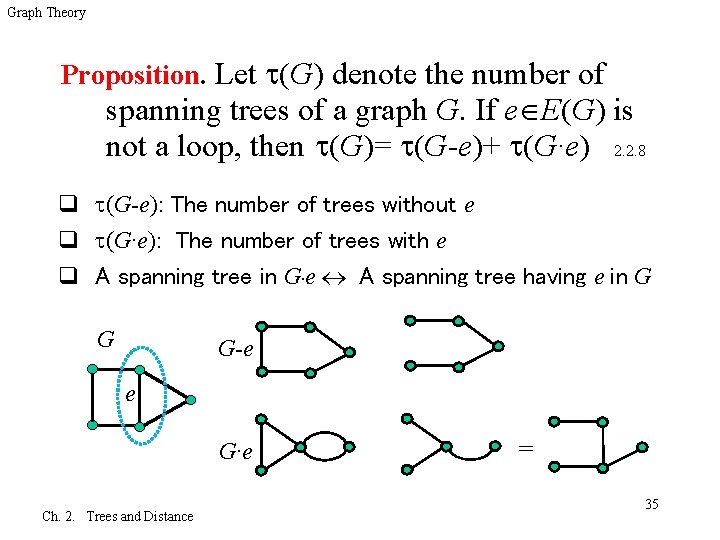
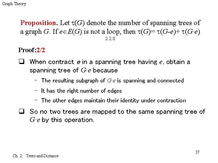
Graph Theory Proposition. Let (G) denote the number of spanning trees of a graph G. If e E(G) is not a loop, then (G)= (G-e)+ (G·e) 2. 2. 8 q (G-e): The number of trees without e q (G·e): The number of trees with e q A spanning tree in G. e A spanning tree having e in G G G-e e G·e Ch. 2. Trees and Distance = 35

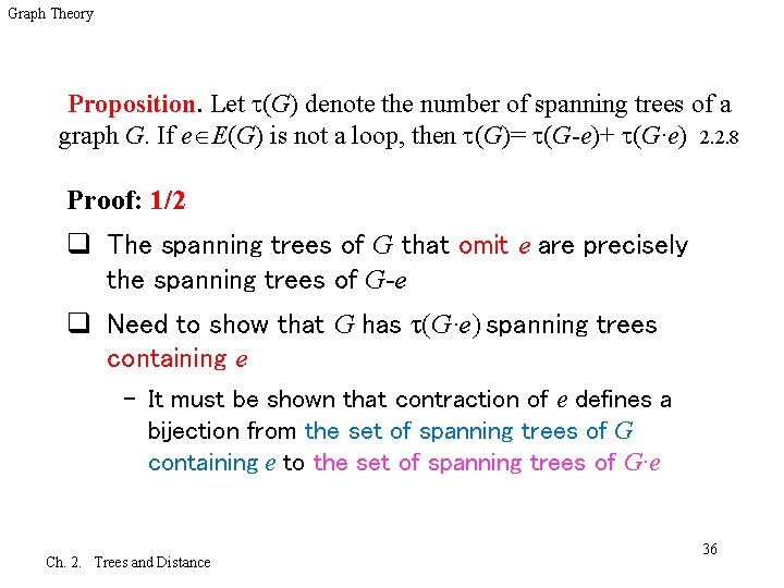
Graph Theory Proposition. Let (G) denote the number of spanning trees of a graph G. If e E(G) is not a loop, then (G)= (G-e)+ (G·e) 2. 2. 8 Proof: 1/2 q The spanning trees of G that omit e are precisely the spanning trees of G-e q Need to show that G has (G·e) spanning trees containing e – It must be shown that contraction of e defines a bijection from the set of spanning trees of G containing e to the set of spanning trees of G·e Ch. 2. Trees and Distance 36

Graph Theory Proposition. Let (G) denote the number of spanning trees of a graph G. If e E(G) is not a loop, then (G)= (G-e)+ (G·e) 2. 2. 8 Proof: 2/2 q When contract e in a spanning tree having e, obtain a spanning tree of G·e because – The resulting subgraph of G·e is spanning and connected – It has the right number of edges – The other edges maintain their identity under contraction q So no two trees are mapped to the same spanning tree of G·e by this operation. Ch. 2. Trees and Distance 37

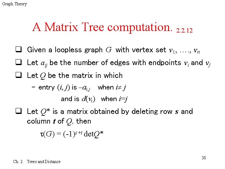
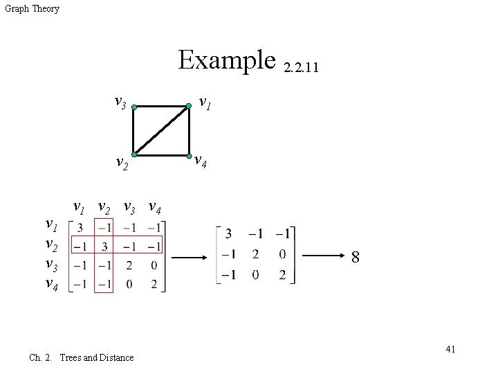
Graph Theory A Matrix Tree computation. 2. 2. 12 q Given a loopless graph G with vertex set v 1, …. , vn q Let aij be the number of edges with endpoints vi and vj q Let Q be the matrix in which – entry (i, j) is –ai, j when i j and is d(vi) when i=j q Let Q* is a matrix obtained by deleting row s and column t of Q, then (G) = (-1)s+t det. Q* Ch. 2. Trees and Distance 38

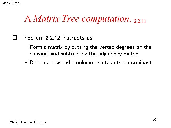
Graph Theory A Matrix Tree computation. 2. 2. 11 q Theorem 2. 2. 12 instructs us – Form a matrix by putting the vertex degrees on the diagonal and subtracting the adjacency matrix – Delete a row and a column and take the eterminant Ch. 2. Trees and Distance 39

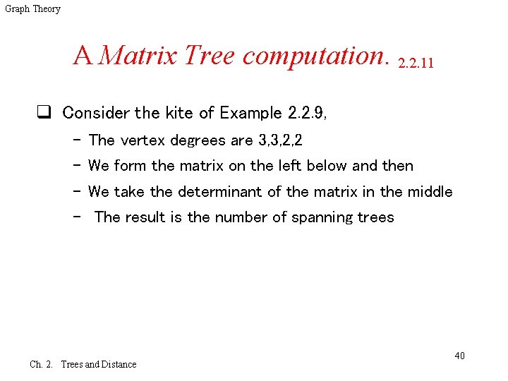
Graph Theory A Matrix Tree computation. 2. 2. 11 q Consider the kite of Example 2. 2. 9, – The vertex degrees are 3, 3, 2, 2 – We form the matrix on the left below and then – We take the determinant of the matrix in the middle – The result is the number of spanning trees Ch. 2. Trees and Distance 40

Graph Theory Example 2. 2. 11 v 2 v 3 v 4 v 3 v 1 v 2 v 4 v 1 v 2 v 3 v 4 Ch. 2. Trees and Distance 8 41

Graph Theory Minimum Spanning Tree 2. 3 q In a connected weighted graph of possible communication links, all spanning trees have n-1 edges; we seek one that minimizes or maximizes the sum of the edge weights. – Kruskal’s Algorithm – Prim’s Algorithm Ch. 2. Trees and Distance 42

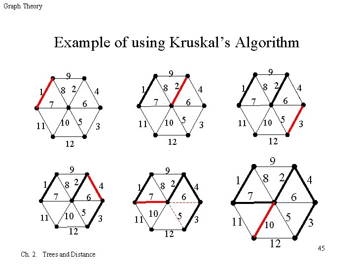
Graph Theory Kruskal’s Algorithm for Minimum Spanning Tree 2. 3. 1 q Input: A weighted connected graph q Idea: – Maintain an acyclic spanning subgraph H. – Enlarging it by edges with low weight to form a spanning tree. – Consider edges in nondecreasing order of weight. Ch. 2. Trees and Distance 43

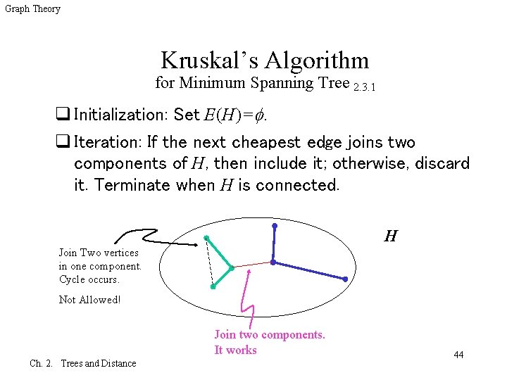
Graph Theory Kruskal’s Algorithm for Minimum Spanning Tree 2. 3. 1 q Initialization: Set E(H)=. q Iteration: If the next cheapest edge joins two components of H, then include it; otherwise, discard it. Terminate when H is connected. H Join Two vertices in one component. Cycle occurs. Not Allowed! Join two components. It works Ch. 2. Trees and Distance 44

Graph Theory Example of using Kruskal’s Algorithm 8 2 1 4 1 3 11 10 5 11 8 2 11 10 5 11 9 9 4 6 10 5 12 Ch. 2. Trees and Distance 3 1 11 8 2 7 10 6 5 12 3 12 12 9 8 2 7 3 4 6 7 6 10 5 12 1 8 2 1 4 7 6 7 9 9 9 4 3 8 2 1 7 11 4 6 10 12 5 3 45

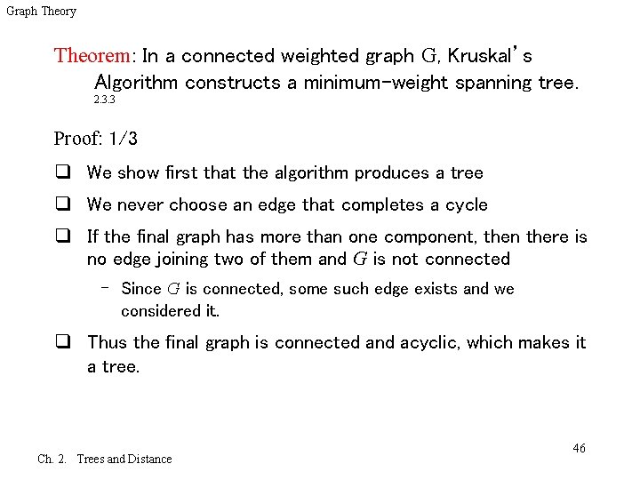
Graph Theory Theorem: In a connected weighted graph G, Kruskal’s Algorithm constructs a minimum-weight spanning tree. 2. 3. 3 Proof: 1/3 q We show first that the algorithm produces a tree q We never choose an edge that completes a cycle q If the final graph has more than one component, then there is no edge joining two of them and G is not connected – Since G is connected, some such edge exists and we considered it. q Thus the final graph is connected and acyclic, which makes it a tree. Ch. 2. Trees and Distance 46

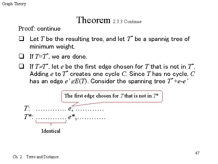
Graph Theory Proof: continue Theorem 2. 3. 3 Continue q Let T be the resulting tree, and let T* be a spannig tree of minimum weight. q If T=T*, we are done. q If T T*, let e be the first edge chosen for T that is not in T*. Adding e to T* creates one cycle C. Since T has no cycle, C has an edge e’ E(T). Consider the spanning tree T*+e-e’ The first edge chosen for T that is not in T* T: …………. e, ………… T*: …………. e*, ………… Identical Ch. 2. Trees and Distance 47

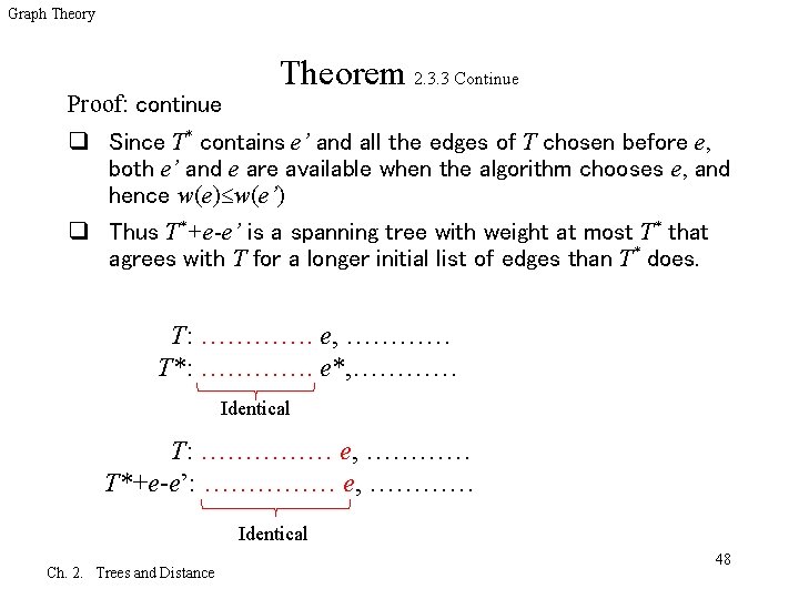
Graph Theory Proof: continue Theorem 2. 3. 3 Continue q Since T* contains e’ and all the edges of T chosen before e, both e’ and e are available when the algorithm chooses e, and hence w(e) w(e’) q Thus T*+e-e’ is a spanning tree with weight at most T* that agrees with T for a longer initial list of edges than T* does. T: …………. e, ………… T*: …………. e*, ………… Identical T: …………… e, ………… T*+e-e’: …………… e, ………… Identical Ch. 2. Trees and Distance 48

Graph Theory Proof: continue Theorem 2. 3. 3 Continue q Repeating this argument eventually yields a minimum-weight spanning tree that agrees completely with T. q Phrased extremely, we have proved that the minimum spanning tree agreeing with T the longest is T itself. Ch. 2. Trees and Distance 49

Graph Theory Shortest Paths q How can we find the shortest route from one location to another? Ch. 2. Trees and Distance 50

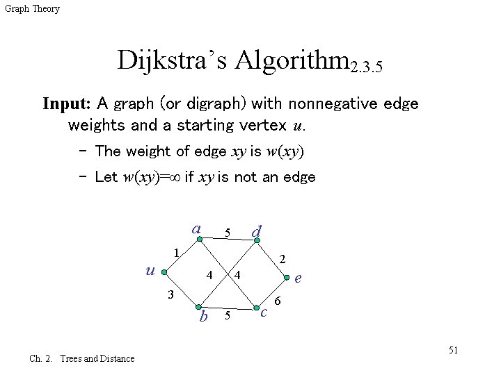
Graph Theory Dijkstra’s Algorithm 2. 3. 5 Input: A graph (or digraph) with nonnegative edge weights and a starting vertex u. – The weight of edge xy is w(xy) – Let w(xy)= if xy is not an edge a d 5 1 u 2 4 4 e 3 b Ch. 2. Trees and Distance 5 c 6 51

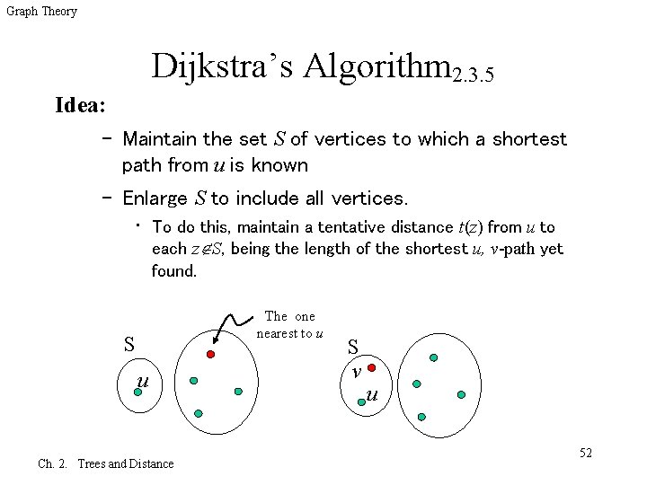
Graph Theory Dijkstra’s Algorithm 2. 3. 5 Idea: – Maintain the set S of vertices to which a shortest path from u is known – Enlarge S to include all vertices. • To do this, maintain a tentative distance t(z) from u to each z S, being the length of the shortest u, v-path yet found. The one nearest to u S u Ch. 2. Trees and Distance S v u 52

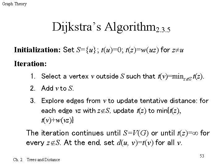
Graph Theory Dijkstra’s Algorithm 2. 3. 5 Initialization: Set S={u}; t(u)=0; t(z)=w(uz) for z u Iteration: 1. Select a vertex v outside S such that t(v)=minz S t(z). 2. Add v to S. 3. Explore edges from v to update tentative distance: for each edge vz with z S, update t(z) to min{t(z), t(v)+w(vz)} The iteration continues until S=V(G) or until t(z)= for every z S. At the end, set d(u, v)=t(v) for all v. Ch. 2. Trees and Distance 53

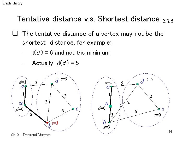
Graph Theory Tentative distance v. s. Shortest distance 2. 3. 5 q The tentative distance of a vertex may not be the shortest distance, for example: – t(d ) = 6 and not the minimum – Actually d(d ) = 5 d=1 d 5 a t=6 d=1 a 1 1 2 u 2 d=0 6 3 b Ch. 2. Trees and Distance t=3 d 5 e t=5 2 u 2 d=0 3 6 e t=9 b d=3 54

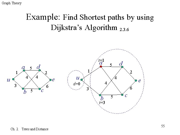
Graph Theory Example: Find Shortest paths by using Dijkstra’s Algorithm 2. 3. 6 t=1 1 u a 5 d 3 5 e c 6 d 5 1 2 4 4 b a 2 u 4 e 4 d=0 6 3 b 5 c t=3 Ch. 2. Trees and Distance 55

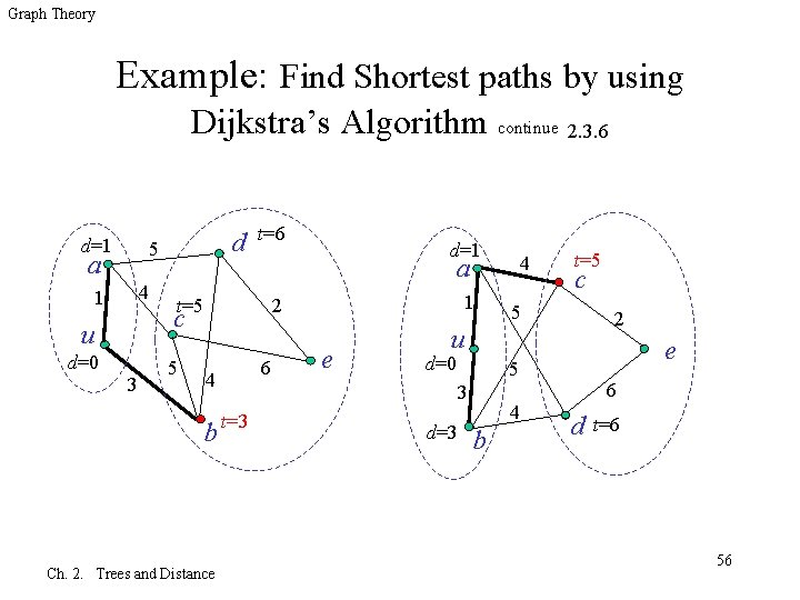
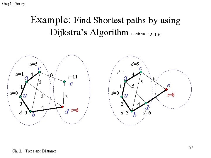
Graph Theory Example: Find Shortest paths by using Dijkstra’s Algorithm continue 2. 3. 6 d=1 d 5 a 4 1 u d=0 3 t=6 1 2 c 6 4 b Ch. 2. Trees and Distance e t=5 c 5 2 u d=0 e 5 3 t=3 4 a t=5 5 d=1 d=3 4 b 6 d t=6 56

Graph Theory Example: Find Shortest paths by using Dijkstra’s Algorithm continue 2. 3. 6 d=5 d=1 a 4 u 5 3 d=3 6 t=11 4 b Ch. 2. Trees and Distance d=1 a e 5 1 d=0 d=5 c 4 u 3 d t=6 6 5 5 1 d=0 2 c d=3 4 b e 2 t=8 d d=6 57

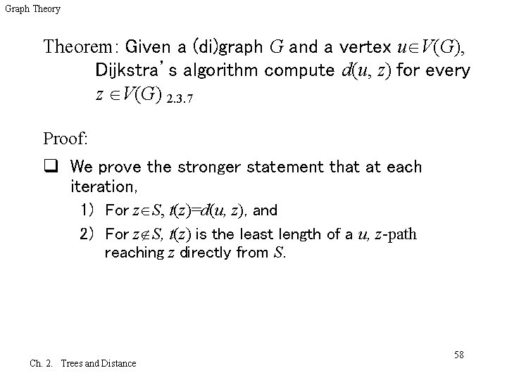
Graph Theory Theorem: Given a (di)graph G and a vertex u V(G), Dijkstra’s algorithm compute d(u, z) for every z V(G) 2. 3. 7 Proof: q We prove the stronger statement that at each iteration, 1) For z S, t(z)=d(u, z), and 2) For z S, t(z) is the least length of a u, z-path reaching z directly from S. Ch. 2. Trees and Distance 58

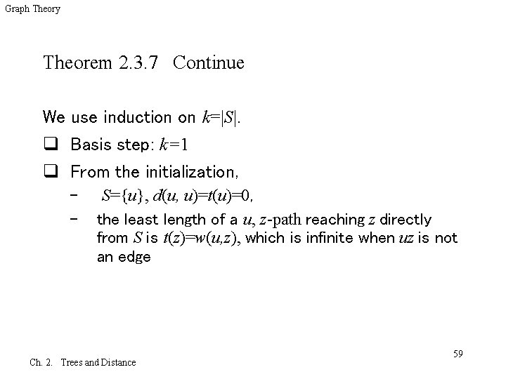
Graph Theory Theorem 2. 3. 7 Continue We use induction on k=|S|. q Basis step: k=1 q From the initialization, – – S={u}, d(u, u)=t(u)=0, the least length of a u, z-path reaching z directly from S is t(z)=w(u, z), which is infinite when uz is not an edge Ch. 2. Trees and Distance 59

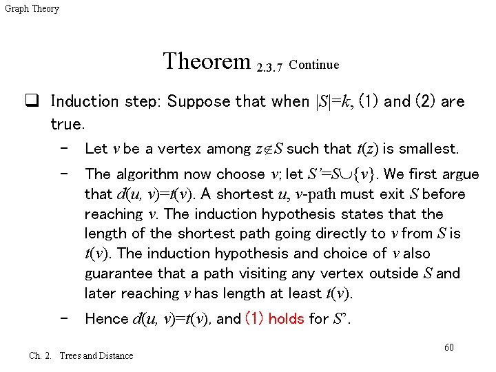
Graph Theory Theorem 2. 3. 7 Continue q Induction step: Suppose that when |S|=k, (1) and (2) are true. – Let v be a vertex among z S such that t(z) is smallest. – The algorithm now choose v; let S’=S {v}. We first argue that d(u, v)=t(v). A shortest u, v-path must exit S before reaching v. The induction hypothesis states that the length of the shortest path going directly to v from S is t(v). The induction hypothesis and choice of v also guarantee that a path visiting any vertex outside S and later reaching v has length at least t(v). – Hence d(u, v)=t(v), and (1) holds for S’. Ch. 2. Trees and Distance 60

Graph Theory Theorem 2. 3. 7 Continue q To prove (2) for S’, let z be a vertex outside S other than v. – By the hypothesis, the shortest u, v-path reaching z directly from S has length t(z) ( if there is no such path). – When we add v to S, we must also consider paths reaching z from v. Since we have now computed d(u, v)=t(v), the shortest such path has length t(v)+w(vz), and we compare this with the previous value of t(z) to find the shortest path reaching z directly from S’. q We have verified that (1) and (2) hold for the new set S’ of size k+1; this completes the induction step. Ch. 2. Trees and Distance 61

Graph Theory Prim’s Algorithm for Minimum Spanning Tree Input: A graph (or digraph) with nonnegtive edge weights and a starting vertex u. The weight of edge xy is w(xy); let w(xy)= if xy is not an edge. Idea: Maintain a tree T including u at the beginning, enlarging T to include all vertices. To do this, select the cheapest edge from the edges E={(x, v) |x T, v T }. Ch. 2. Trees and Distance 62

Graph Theory Prim’s Algorithm Initialization: Set T={u}. Iteration: – Select a vertex v outside T such that w(x, v)=minx T, v T w(x, v) – Add v to T – The iteration continues until V(T )=V(G). Ch. 2. Trees and Distance 63

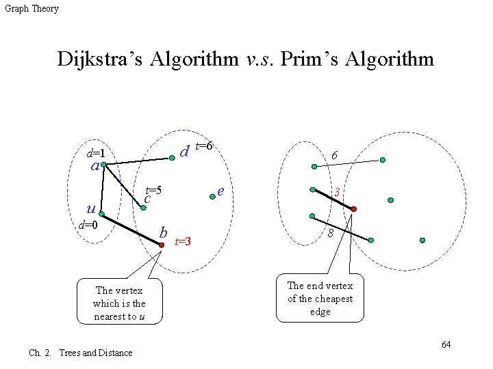
Graph Theory Dijkstra’s Algorithm v. s. Prim’s Algorithm d d=1 a c d=0 The vertex which is the nearest to u Ch. 2. Trees and Distance b 6 e t=5 u t=6 t=3 3 8 The end vertex of the cheapest edge 64

Graph Theory Algorithm - Breadth First Search 2. 3. 8 Input: An unweighted graph (or digraph) and a start vertex u. Idea: Maintain a set R of vertices that have been reached but not searched and a set S of vertices that have been searched The set R is maintained as a First-In First-Out list (queue), so the first vertices found are the first vertices explored Ch. 2. Trees and Distance 65

Graph Theory Algorithm - Breadth First Search 2. 3. 8 Initialization: R={u}, S= , d(u, u)=0 Iteration: 1. As long as R , we search from the first vertex v of R 2. The neighbors of v not in S R are added to the back of R and assigned distance d(u, v)+1 3. Then v is removed from the front of R and placed in S Ch. 2. Trees and Distance 66

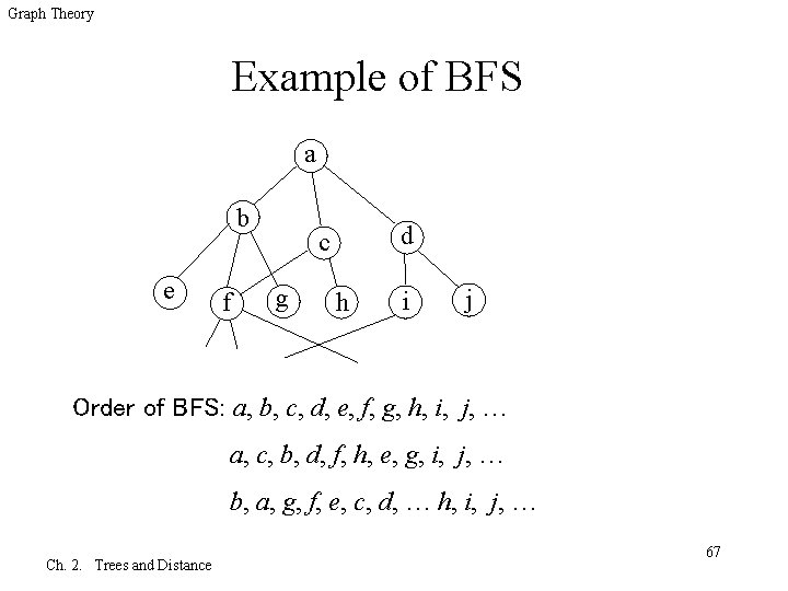
Graph Theory Example of BFS a b e f d c g h i j Order of BFS: a, b, c, d, e, f, g, h, i, j, … a, c, b, d, f, h, e, g, i, j, … b, a, g, f, e, c, d, … h, i, j, … Ch. 2. Trees and Distance 67

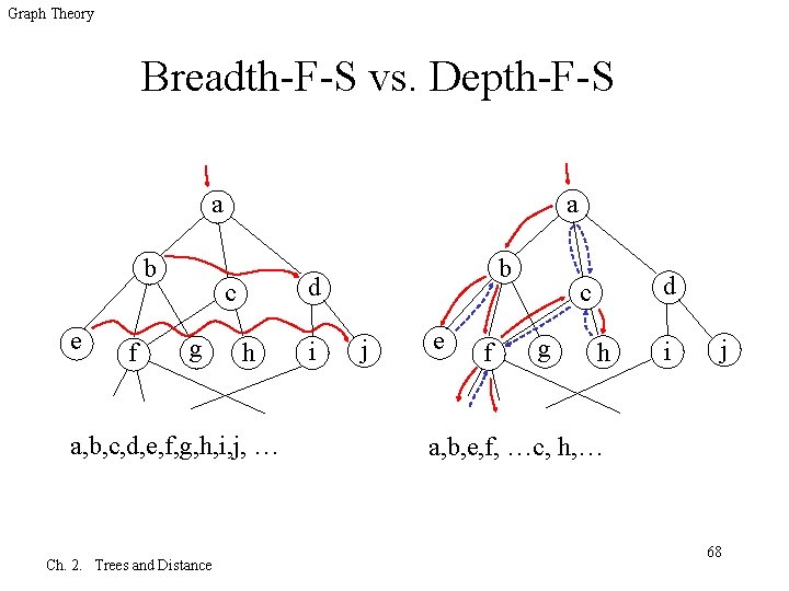
Graph Theory Breadth-F-S vs. Depth-F-S a a b e f d c g h a, b, c, d, e, f, g, h, i, j, … Ch. 2. Trees and Distance b i j e f d c g h i j a, b, e, f, …c, h, … 68

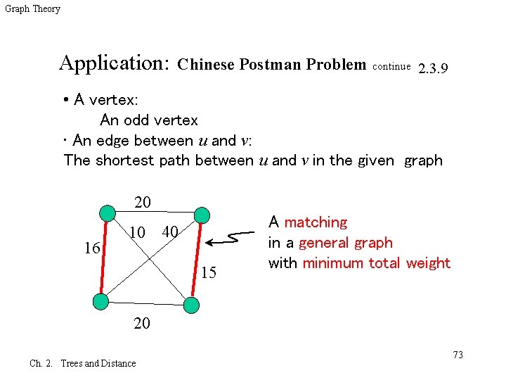
Graph Theory Application: Chinese Postman Problem 2. 3. 9 q A mail carrier must traverse all edges in a road network, starting and ending at the Post Office. – The edges has nonnegative weights representing distance or time. – We seek a closed walk of minimum total length that uses all the edges – This is the Chinese Postman Problem, • named in honor of the Chinese mathematician Guan Meigu [1962], who proposed it. Ch. 2. Trees and Distance 69

Graph Theory Application: Chinese Postman Problem continue 2. 3. 9 q If every vertex is even, then the graph is Eulerian and the answer is the sum of the edge weights. q Otherwise, we must repeat edges. Every traversal is an Eulerian circuit of a graph obtained by duplicating edges. q Finding the shortest traversal is equivalent to finding the minimum total weight of edges whose duplication will make all vertex degrees even. Ch. 2. Trees and Distance 70

Graph Theory Application: Chinese Postman Problem continue 2. 3. 9 q We say “duplication” because we need not use an edge more than twice q If we use an edge three or more times in making all vertices even, then deleting two of those copies will leave all vertices even q There may be many ways to choose the duplicated edges Ch. 2. Trees and Distance 71

Graph Theory Application: Chinese Postman Problem continue 2. 3. 9 q If there are only two odd vertices, then – We can use Dijkstra’s Algorithm to find the shortest path between them and solve the problem q If there are 2 k odd vertices, then – Use Dijkstra’s algorithm to find the shortest paths connecting each pair of odd vertices – Use these lengths as weights on the edges of K 2 k – Find the minimum total weight of k edges that pair up these 2 k vertices. This is a maximum matching problem. Ch. 2. Trees and Distance 72

Graph Theory Application: Chinese Postman Problem continue 2. 3. 9 • A vertex: An odd vertex • An edge between u and v: The shortest path between u and v in the given graph 20 16 10 40 15 A matching in a general graph with minimum total weight 20 Ch. 2. Trees and Distance 73

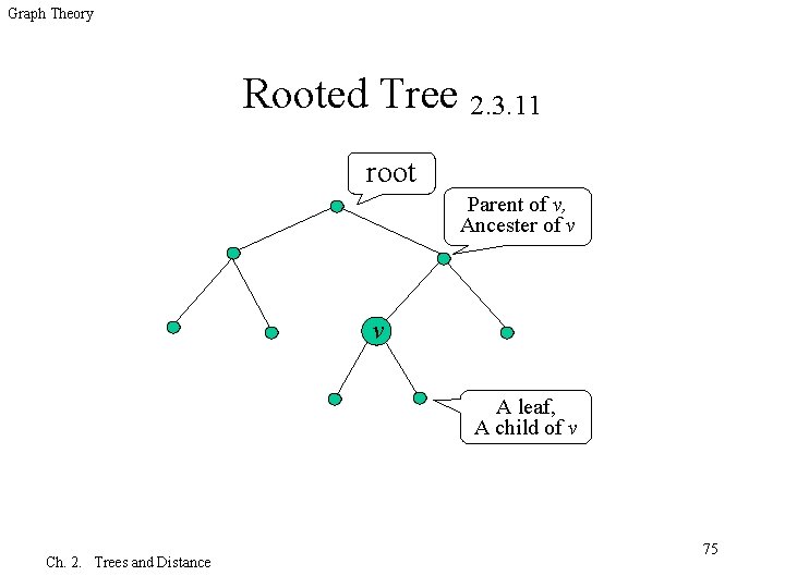
Graph Theory Rooted Tree 2. 3. 11 q A rooted tree is a tree with one vertex r chosen as root. q For each vertex v, let P(v) be the unique v, r-path. – The parent of v is its neighbor on P(v); – Its children are its other neighbors. – Its ancestors are the vertices of P(v)-v. – Its descendants are the vertices u such that P(u) contains v. – The leaves are the vertices with no children. – A rooted plane tree or planted tree is a rooted tree with a left -to–right ordering specified for the children of each vertex. Ch. 2. Trees and Distance 74

Graph Theory Rooted Tree 2. 3. 11 root Parent of v, Ancester of v v A leaf, A child of v Ch. 2. Trees and Distance 75

Graph Theory Binary Tree 2. 3. 12 q A binary tree is a rooted plane tree where each vertex has at most two children, and each child of a vertex is designated as its left child or right child q The subtrees rooted at the children of the root are the left subtree and the right subtree of the tree q A k-ary tree allows each vertex up to k children Ch. 2. Trees and Distance 76

Graph Theory Huffman’s Algorithm 2. 3. 13 Input: Weights (frequencies or probabilities) p 1, …, pn Output: Prefix-free code (equivalently, a binary tree) Idea: Infrequent items should have longer codes; put infrequent items deeper by combining them into parent nodes Ch. 2. Trees and Distance 77

Graph Theory Huffman’s Algorithm 2. 3. 13 Initial case: When n=2, the optimal length is one, with 0 and 1 being the codes assigned to the two items (the tree has a root and two leaves; n=1 can also be used as the initial case) Ch. 2. Trees and Distance 78

Graph Theory Huffman’s Algorithm 2. 3. 13 Recursion: q Replace the two least likely items p, p’ with a single item q of weight p+p’ when n>2 q Treat the smaller set as a problem with n-1 items. q After solving it, give children with weights p, p’ to the resulting leaf with weight q. – Equivalently, replace the code computed for the combined item with its extensions by 1 and 0, assigned to the items that were replaced. Ch. 2. Trees and Distance 79

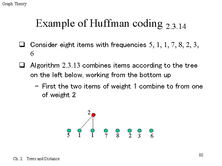
Graph Theory Example of Huffman coding 2. 3. 14 q Consider eight items with frequencies 5, 1, 1, 7, 8, 2, 3, 6 q Algorithm 2. 3. 13 combines items according to the tree on the left below, working from the bottom up – First the two items of weight 1 combine to from one of weight 2 2 5 Ch. 2. Trees and Distance 1 1 7 8 2 3 6 80

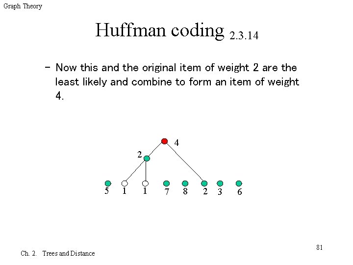
Graph Theory Huffman coding 2. 3. 14 – Now this and the original item of weight 2 are the least likely and combine to form an item of weight 4. 4 2 5 Ch. 2. Trees and Distance 1 1 7 8 2 3 6 81

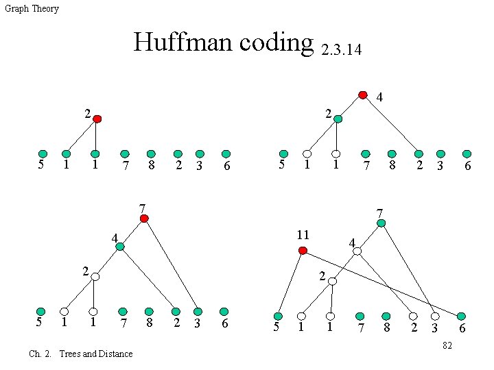
Graph Theory Huffman coding 2. 3. 14 4 2 5 1 2 1 8 7 2 3 6 5 1 1 7 11 2 3 6 7 4 5 8 7 4 2 1 7 Ch. 2. Trees and Distance 8 2 3 6 5 1 1 7 8 2 3 6 82

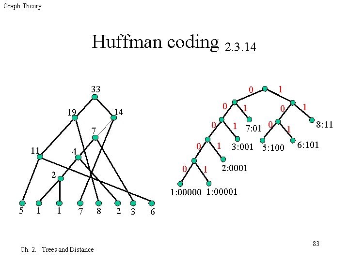
Graph Theory Huffman coding 2. 3. 14 33 0 0 14 19 11 1 0 4 0 2 1 1 0 1 7: 01 0 0 7 1 1 3: 001 5: 100 1 8: 11 6: 101 2: 0001 1: 00000 1: 00001 5 1 1 7 Ch. 2. Trees and Distance 8 2 3 6 83

Graph Theory Theorem 2. 3. 15 q Given a probability distribution {pi} on n items, Huffman’s Algorithm produces the prefix-free code with minimum excepted length Ch. 2. Trees and Distance 84