Spectral Graph Theory and its Applications Daniel A

Spectral Graph Theory and its Applications Daniel A. Spielman Dept. of Computer Science Program in Applied Mathematics Yale Unviersity

Outline Adjacency matrix and Laplacian Intuition, spectral graph drawing Physical intuition Isomorphism testing Random walks Graph Partitioning and clustering Distributions of eigenvalues and compression Computation

What I’m Skipping Matrix-tree theorem. Most of algebraic graph theory. Special graphs (e. g. Cayley graphs). Connections to codes and designs. Lots of work by theorists. Expanders.

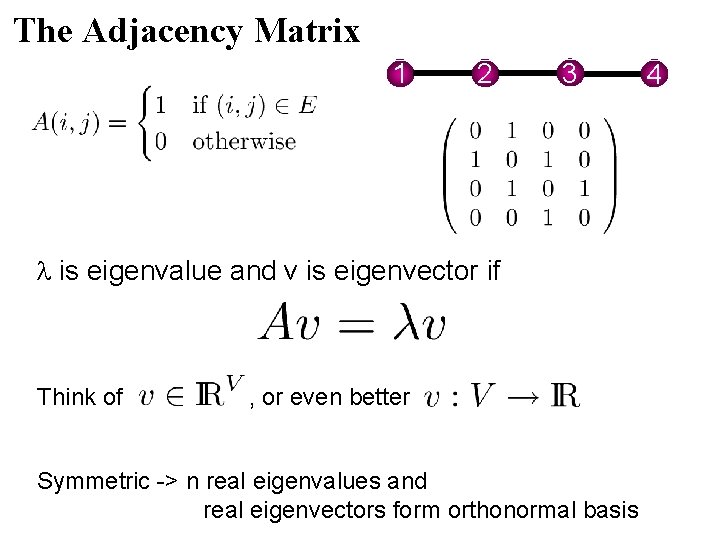
The Adjacency Matrix 1 2 3 is eigenvalue and v is eigenvector if Think of , or even better Symmetric -> n real eigenvalues and real eigenvectors form orthonormal basis 4

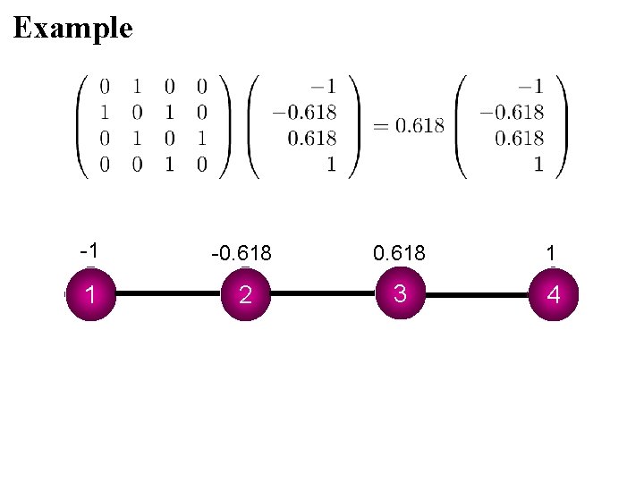
Example -1 -0. 618 1 1 2 3 4

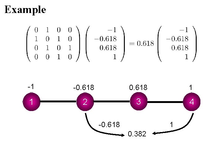
Example -1 -0. 618 1 1 2 3 4 -0. 618 1 0. 382

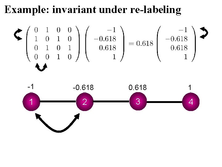
Example: invariant under re-labeling -1 -0. 618 1 1 2 3 4

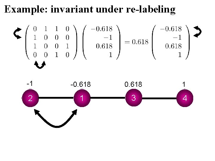
Example: invariant under re-labeling -1 -0. 618 1 2 1 3 4

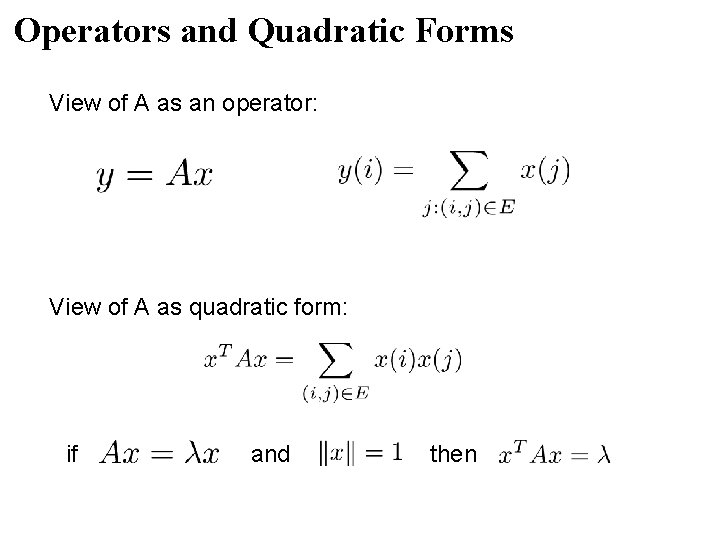
Operators and Quadratic Forms View of A as an operator: View of A as quadratic form: if and then

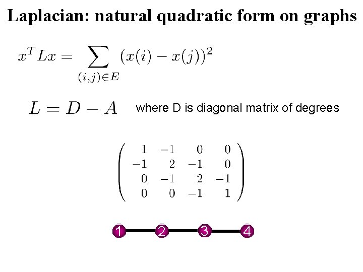
Laplacian: natural quadratic form on graphs where D is diagonal matrix of degrees 1 2 3 4

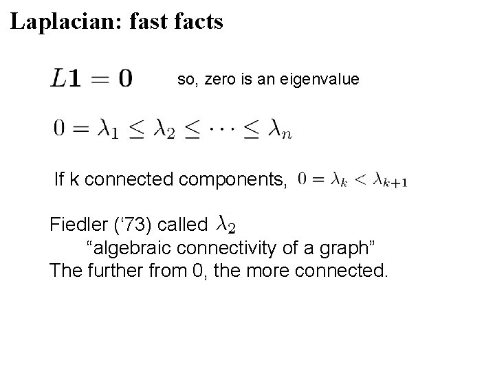
Laplacian: fast facts so, zero is an eigenvalue If k connected components, Fiedler (‘ 73) called “algebraic connectivity of a graph” The further from 0, the more connected.

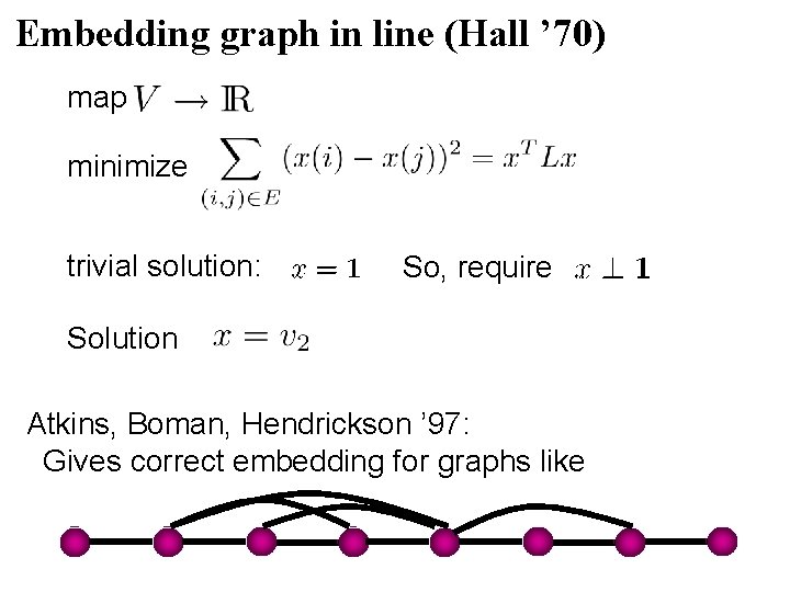
Embedding graph in line (Hall ’ 70) map minimize trivial solution: So, require Solution Atkins, Boman, Hendrickson ’ 97: Gives correct embedding for graphs like

Courant-Fischer definition of eigvals/vecs (here )

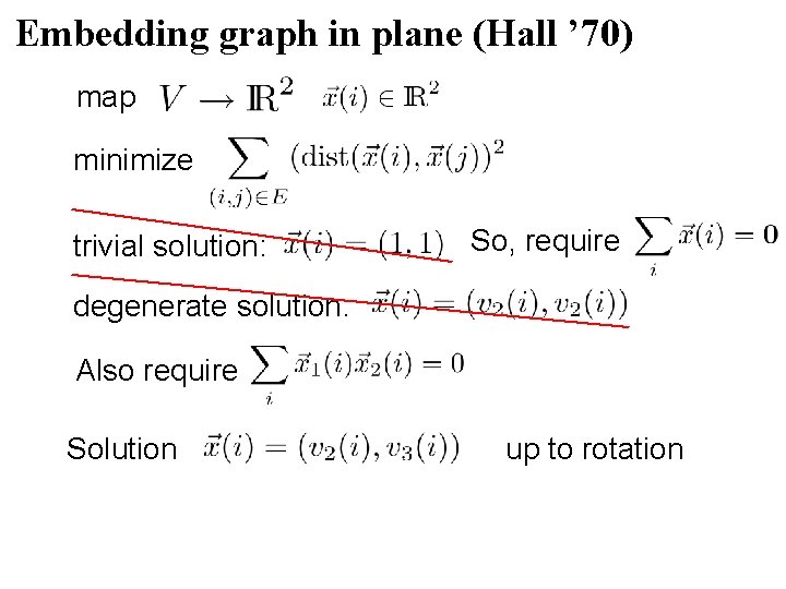
Embedding graph in plane (Hall ’ 70) map minimize trivial solution: So, require degenerate solution: Also require Solution up to rotation

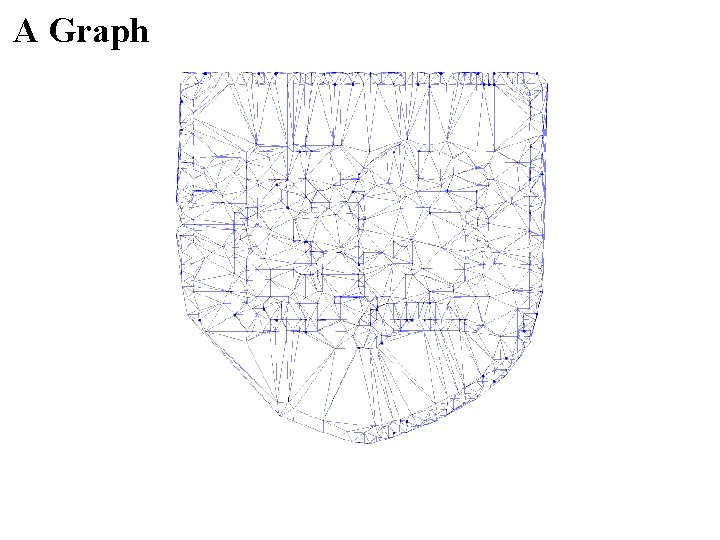
A Graph

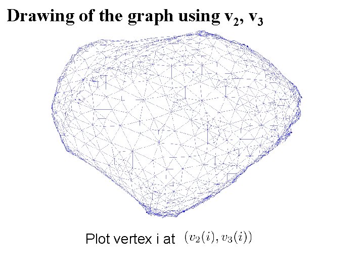
Drawing of the graph using v 2, v 3 Plot vertex i at

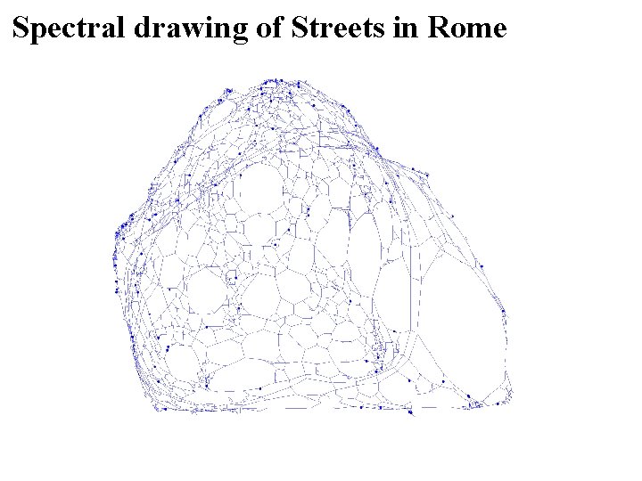
Spectral drawing of Streets in Rome

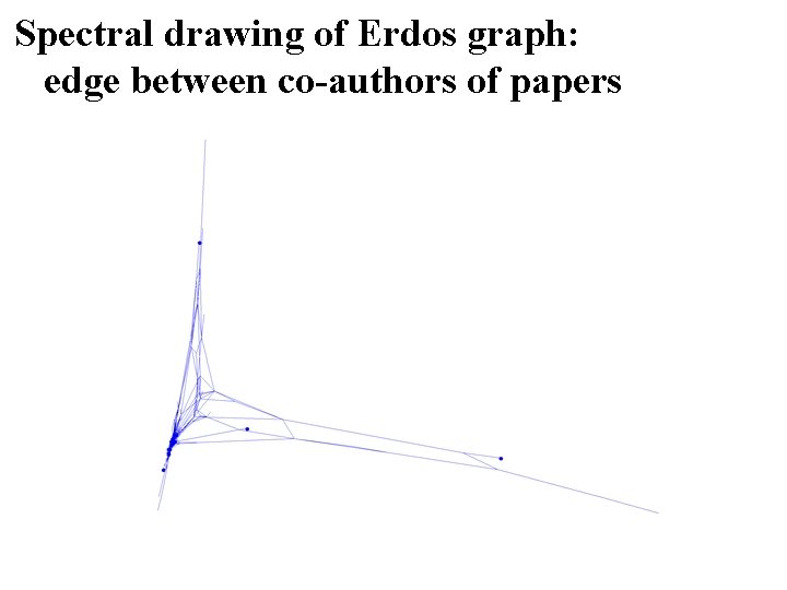
Spectral drawing of Erdos graph: edge between co-authors of papers

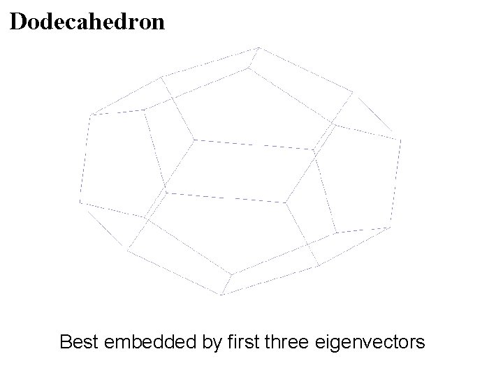
Dodecahedron Best embedded by first three eigenvectors

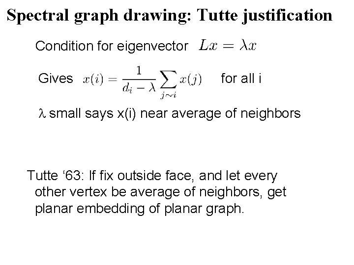
Spectral graph drawing: Tutte justification Condition for eigenvector Gives for all i small says x(i) near average of neighbors Tutte ‘ 63: If fix outside face, and let every other vertex be average of neighbors, get planar embedding of planar graph.

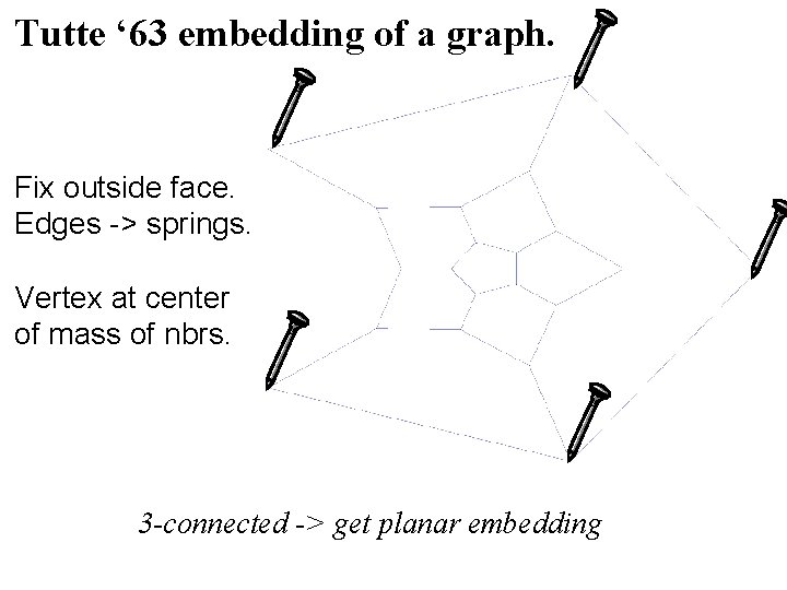
Tutte ‘ 63 embedding of a graph. Fix outside face. Edges -> springs. Vertex at center of mass of nbrs. 3 -connected -> get planar embedding

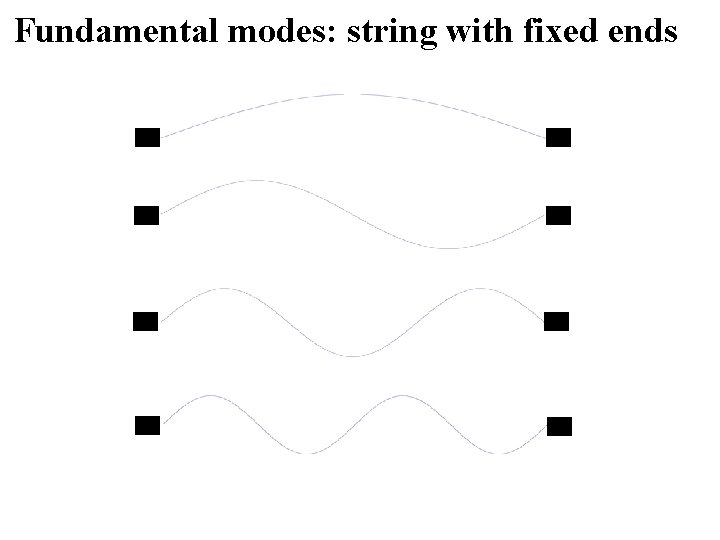
Fundamental modes: string with fixed ends

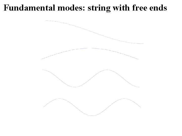
Fundamental modes: string with free ends

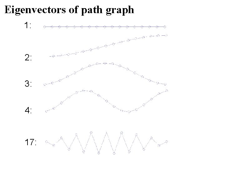
Eigenvectors of path graph 1: 2: 3: 4: 17:

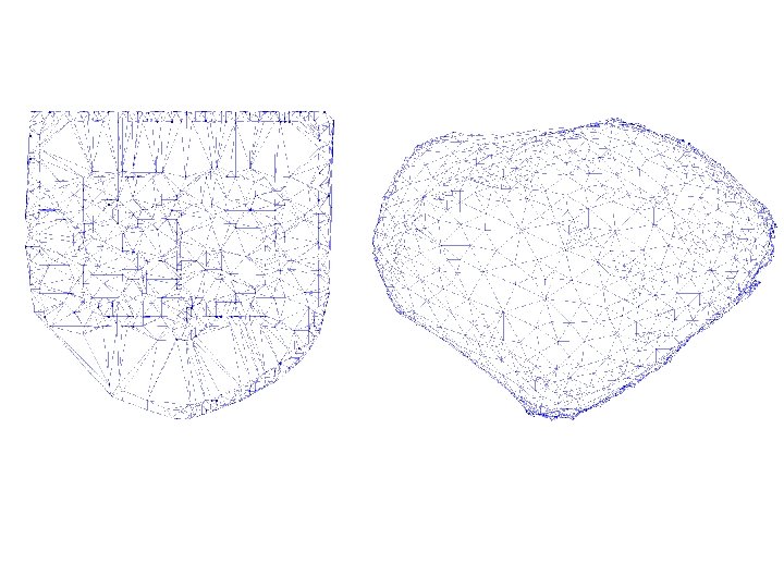
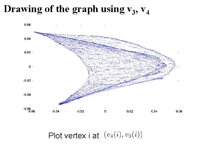
Drawing of the graph using v 3, v 4 Plot vertex i at

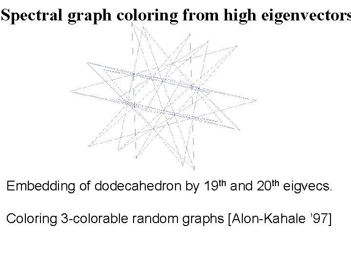
Spectral graph coloring from high eigenvectors Embedding of dodecahedron by 19 th and 20 th eigvecs. Coloring 3 -colorable random graphs [Alon-Kahale ’ 97]

Spectral graph drawing: FEM justification If apply finite element method to solve Laplace’s equation in the plane with a Delaunay triangulation Would get graph Laplacian, but with some weights on edges Fundamental solutions are x and y coordinates (see Strang’s Introduction to Applied Mathematics)

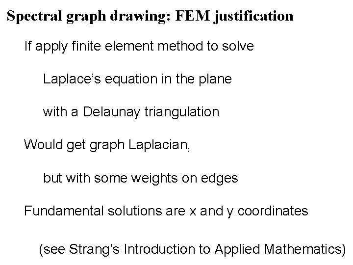
Isomorphism testing 1. different eigenvalues -> non-isomorphic 2. If each vertex distinct in spectral embedding, just need to line up embeddings. Each eigvec determined up to sign.

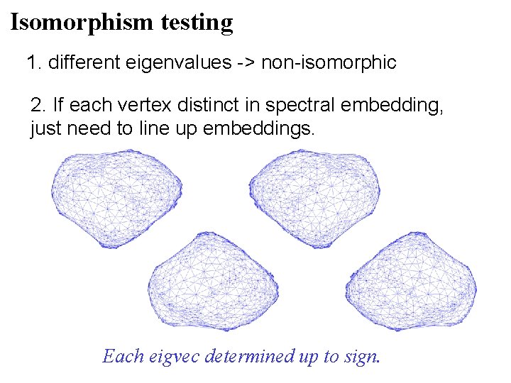
Isomorphism testing 2 = 3, eigvecs determined up to rotation

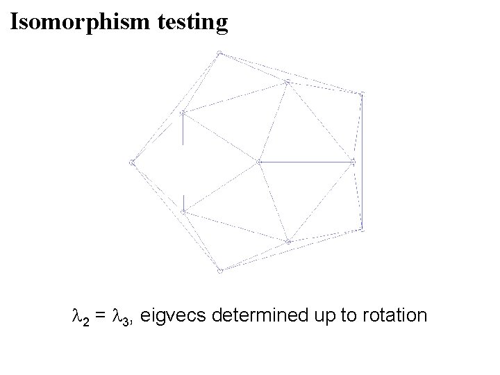
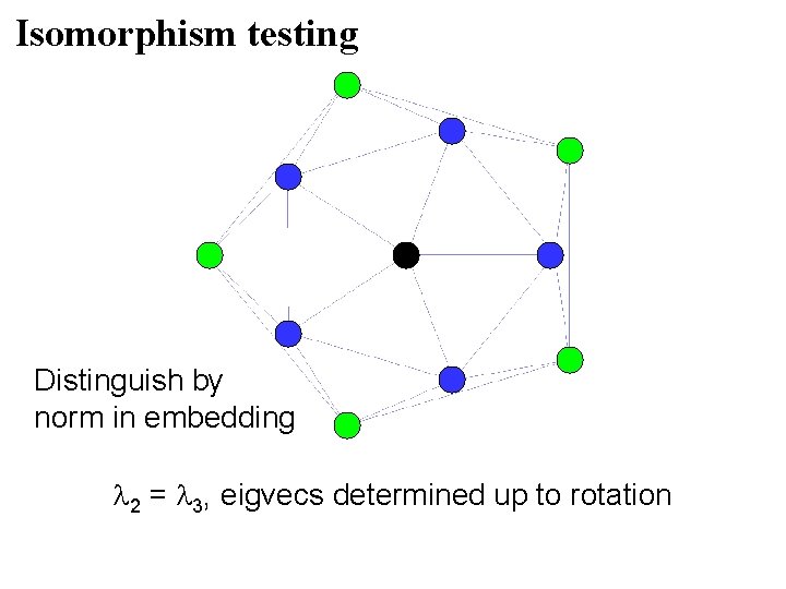
Isomorphism testing Distinguish by norm in embedding 2 = 3, eigvecs determined up to rotation

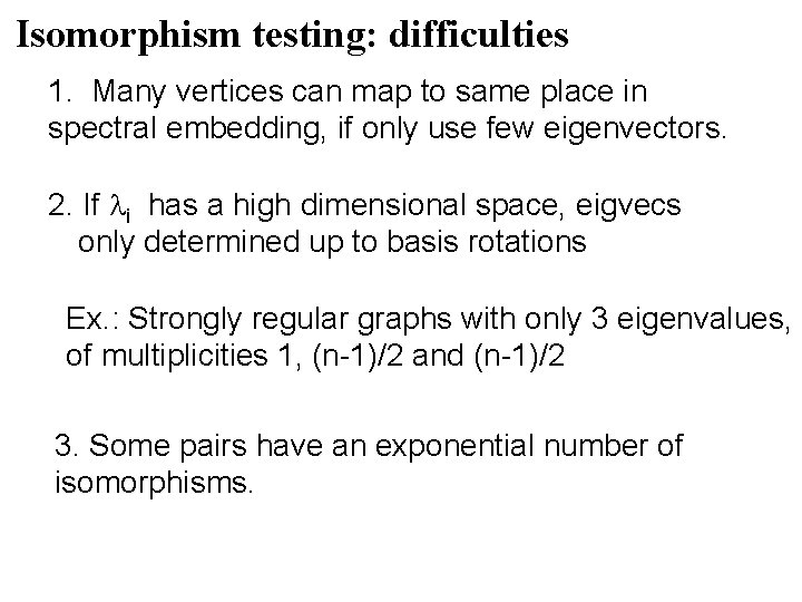
Isomorphism testing: difficulties 1. Many vertices can map to same place in spectral embedding, if only use few eigenvectors. 2. If i has a high dimensional space, eigvecs only determined up to basis rotations Ex. : Strongly regular graphs with only 3 eigenvalues, of multiplicities 1, (n-1)/2 and (n-1)/2 3. Some pairs have an exponential number of isomorphisms.

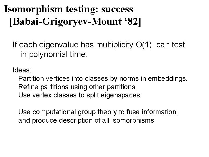
Isomorphism testing: success [Babai-Grigoryev-Mount ‘ 82] If each eigenvalue has multiplicity O(1), can test in polynomial time. Ideas: Partition vertices into classes by norms in embeddings. Refine partitions using other partitions. Use vertex classes to split eigenspaces. Use computational group theory to fuse information, and produce description of all isomorphisms.

Random Walks

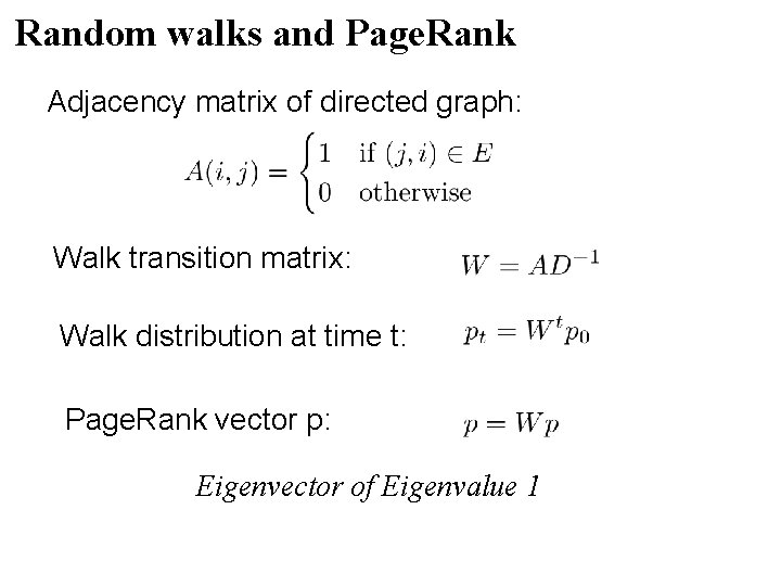
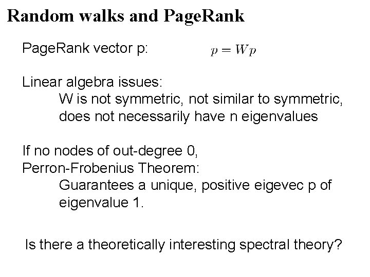
Random walks and Page. Rank Adjacency matrix of directed graph: Walk transition matrix: Walk distribution at time t: Page. Rank vector p: Eigenvector of Eigenvalue 1

Random walks and Page. Rank vector p: Linear algebra issues: W is not symmetric, not similar to symmetric, does not necessarily have n eigenvalues If no nodes of out-degree 0, Perron-Frobenius Theorem: Guarantees a unique, positive eigevec p of eigenvalue 1. Is there a theoretically interesting spectral theory?

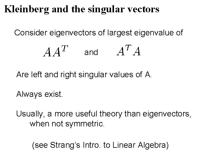
Kleinberg and the singular vectors Consider eigenvectors of largest eigenvalue of and Are left and right singular values of A. Always exist. Usually, a more useful theory than eigenvectors, when not symmetric. (see Strang’s Intro. to Linear Algebra)

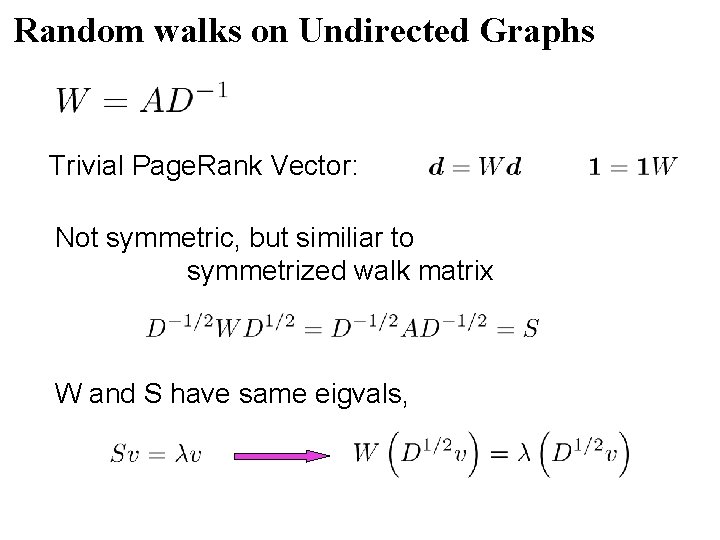
Random walks on Undirected Graphs Trivial Page. Rank Vector: Not symmetric, but similiar to symmetrized walk matrix W and S have same eigvals,

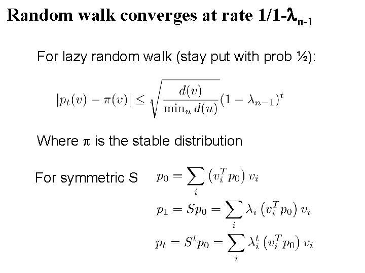
Random walk converges at rate 1/1 - n-1 For lazy random walk (stay put with prob ½): Where is the stable distribution For symmetric S

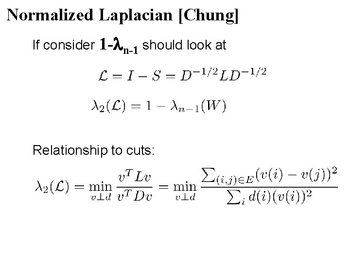
Normalized Laplacian [Chung] If consider 1 - n-1 should look at Relationship to cuts:

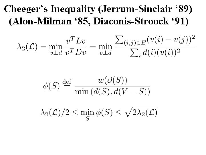
Cheeger’s Inequality (Jerrum-Sinclair ‘ 89) (Alon-Milman ‘ 85, Diaconis-Stroock ‘ 91)

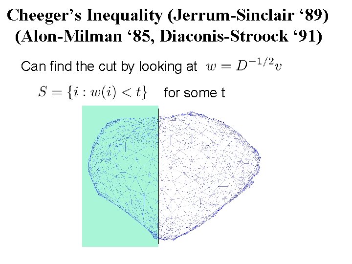
Cheeger’s Inequality (Jerrum-Sinclair ‘ 89) (Alon-Milman ‘ 85, Diaconis-Stroock ‘ 91) Can find the cut by looking at for some t

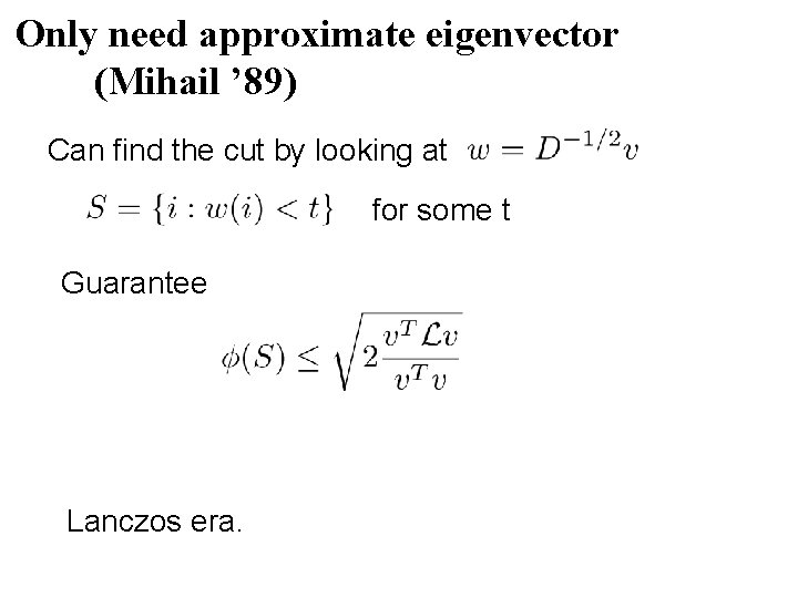
Only need approximate eigenvector (Mihail ’ 89) Can find the cut by looking at for some t Guarantee Lanczos era.

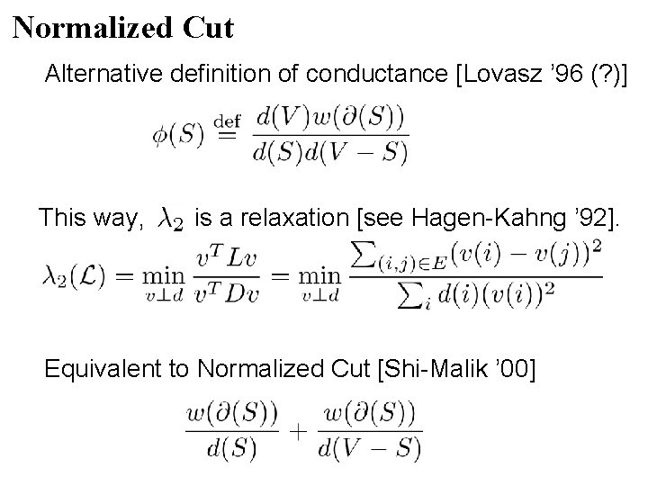
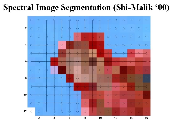
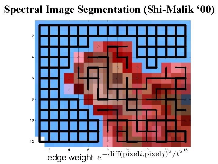
Normalized Cut Alternative definition of conductance [Lovasz ’ 96 (? )] This way, is a relaxation [see Hagen-Kahng ’ 92]. Equivalent to Normalized Cut [Shi-Malik ’ 00]

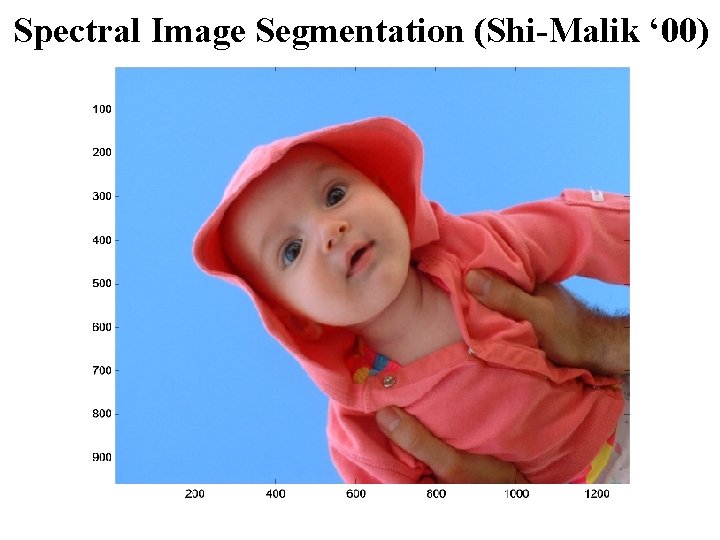
Spectral Image Segmentation (Shi-Malik ‘ 00)

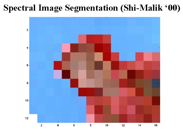
Spectral Image Segmentation (Shi-Malik ‘ 00)

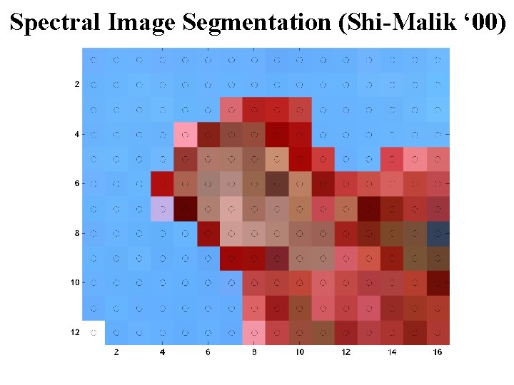
Spectral Image Segmentation (Shi-Malik ‘ 00)

Spectral Image Segmentation (Shi-Malik ‘ 00)

Spectral Image Segmentation (Shi-Malik ‘ 00) edge weight

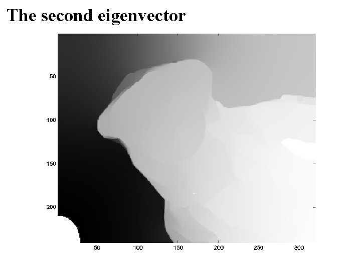
The second eigenvector

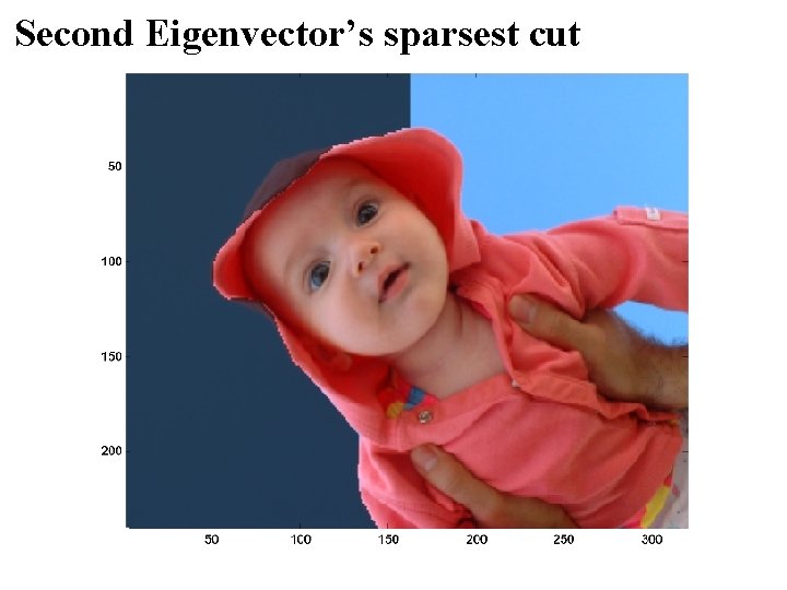
Second Eigenvector’s sparsest cut

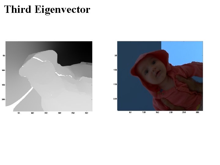
Third Eigenvector

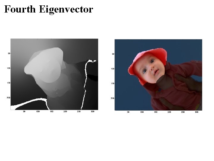
Fourth Eigenvector

Perspective on Spectral Image Segmentation Ignoring a lot we know about images. On non-image data, gives good intuition. Can we fuse with what we know about images? Generally, can we fuse with other knowledge? What about better cut algorithms?

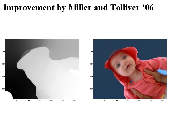
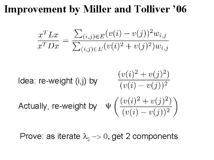
Improvement by Miller and Tolliver ’ 06

Improvement by Miller and Tolliver ’ 06 Idea: re-weight (i, j) by Actually, re-weight by Prove: as iterate 2 -> 0, get 2 components

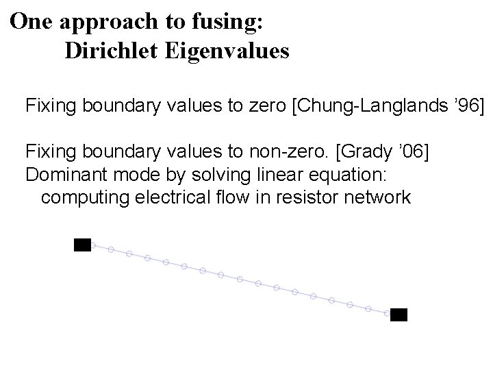
One approach to fusing: Dirichlet Eigenvalues Fixing boundary values to zero [Chung-Langlands ’ 96] Fixing boundary values to non-zero. [Grady ’ 06] Dominant mode by solving linear equation: computing electrical flow in resistor network

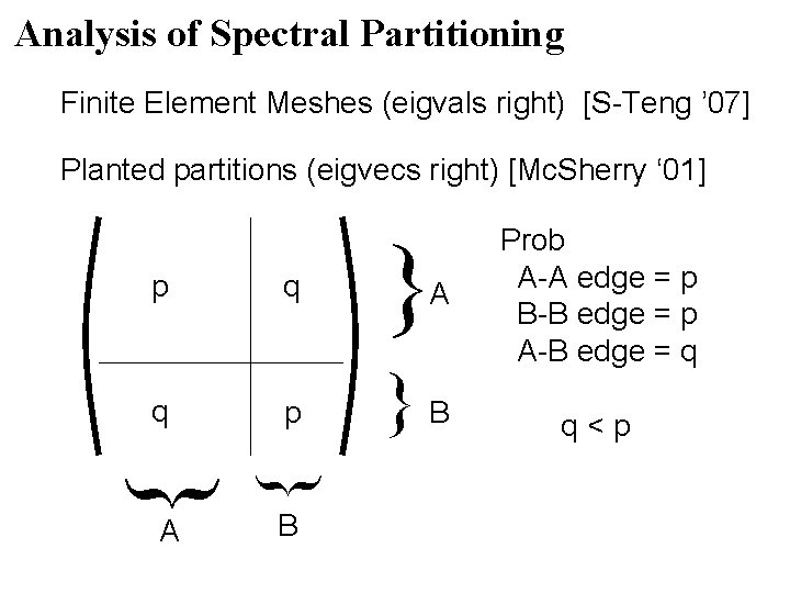
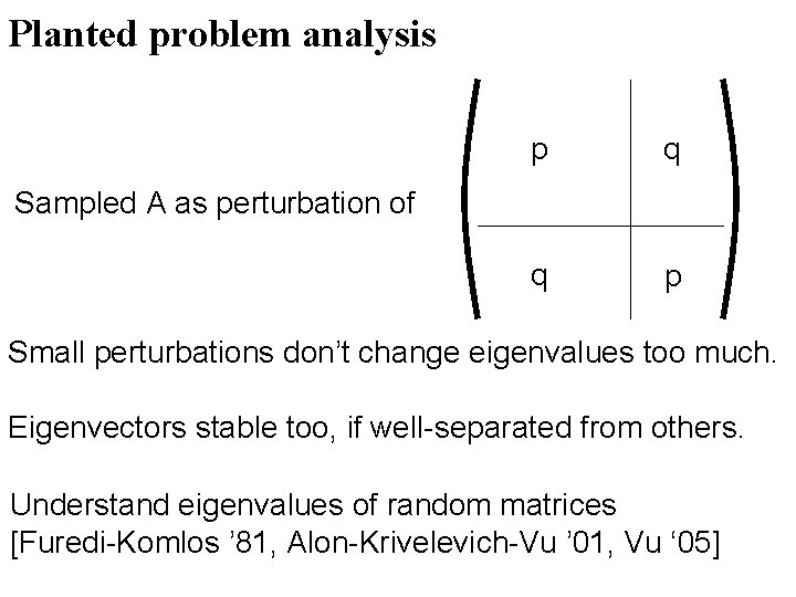
Analysis of Spectral Partitioning Finite Element Meshes (eigvals right) [S-Teng ’ 07] Planted partitions (eigvecs right) [Mc. Sherry ‘ 01] p q } q p }B } } A B A Prob A-A edge = p B-B edge = p A-B edge = q q<p

Other planted problems Finding cn 1/2 clique in random graph [Alon-Krivelevich-Sudakov ’ 98] Color random sparse k-colorable graph [Alon-Kahale ’ 97] Asymmetric block structure (LSI and HITS) [Azar-Fiat-Karlin-Mc. Sherry-Saia ’ 01] Partitioning with widely varying degrees [Dasgupta-Hopcroft-Mc. Sherry ’ 04]

Planted problem analysis p q q p Sampled A as perturbation of Small perturbations don’t change eigenvalues too much. Eigenvectors stable too, if well-separated from others. Understand eigenvalues of random matrices [Furedi-Komlos ’ 81, Alon-Krivelevich-Vu ’ 01, Vu ‘ 05]

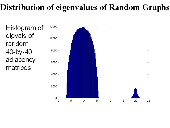
Distribution of eigenvalues of Random Graphs Histogram of eigvals of random 40 -by-40 adjacency matrices

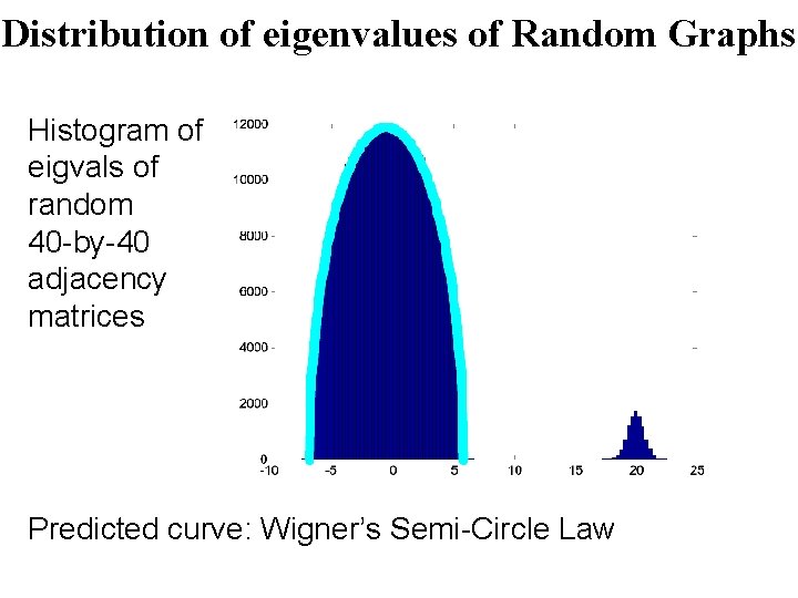
Distribution of eigenvalues of Random Graphs Histogram of eigvals of random 40 -by-40 adjacency matrices Predicted curve: Wigner’s Semi-Circle Law

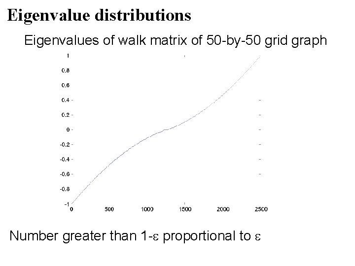
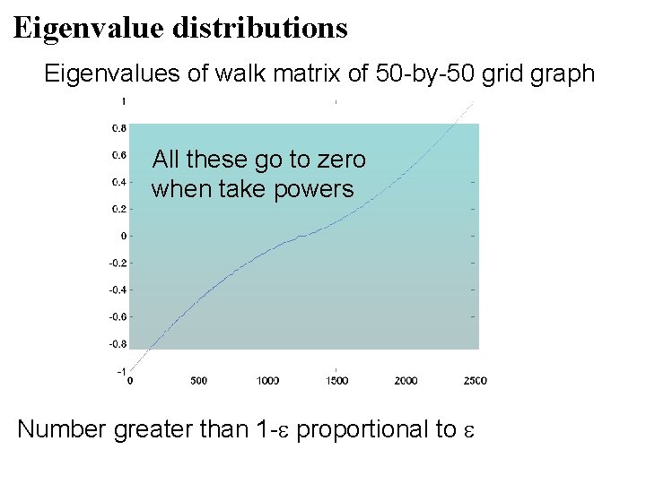
Eigenvalue distributions Eigenvalues of walk matrix of 50 -by-50 grid graph Number greater than 1 - proportional to

Eigenvalue distributions Eigenvalues of walk matrix of 50 -by-50 grid graph All these go to zero when take powers Number greater than 1 - proportional to

Compression of powers of graphs [Coifman, Lafon, Lee, Maggioni, Nadler, Warner, Zucker ’ 05] If most eigenvalues of A and W bounded from 1. Most eigenvalues of At very small. Can approximate At by low-rank matrix. Build wavelets bases on graphs. Solve linear equations and compute eigenvectors. Make rigorous by taking graph from discretization of manifold

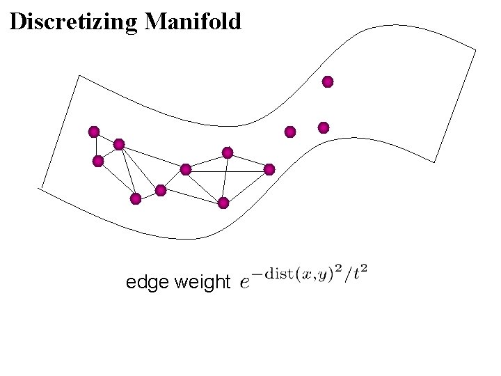
Discretizing Manifold edge weight

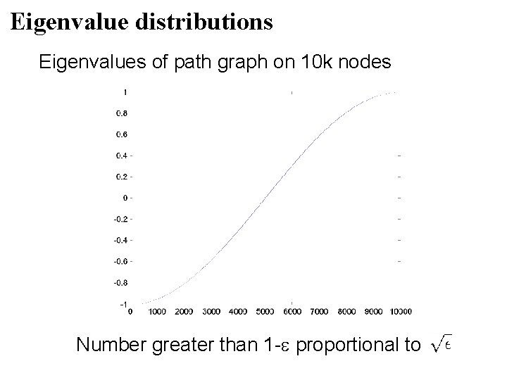
Eigenvalue distributions Eigenvalues of path graph on 10 k nodes Number greater than 1 - proportional to

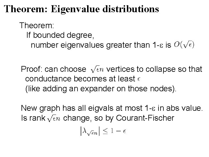
Theorem: Eigenvalue distributions Theorem: If bounded degree, number eigenvalues greater than 1 - is Proof: can choose vertices to collapse so that conductance becomes at least (like adding an expander on those nodes). New graph has all eigvals at most 1 - in abs value. Is rank change, so by Courant-Fischer

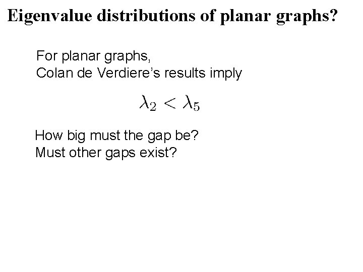
Eigenvalue distributions of planar graphs? For planar graphs, Colan de Verdiere’s results imply How big must the gap be? Must other gaps exist?

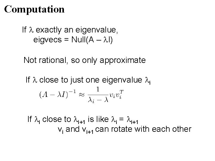
Computation If exactly an eigenvalue, eigvecs = Null(A – I) Not rational, so only approximate If close to just one eigenvalue i If i close to i+1 is like i = i+1 vi and vi+1 can rotate with each other

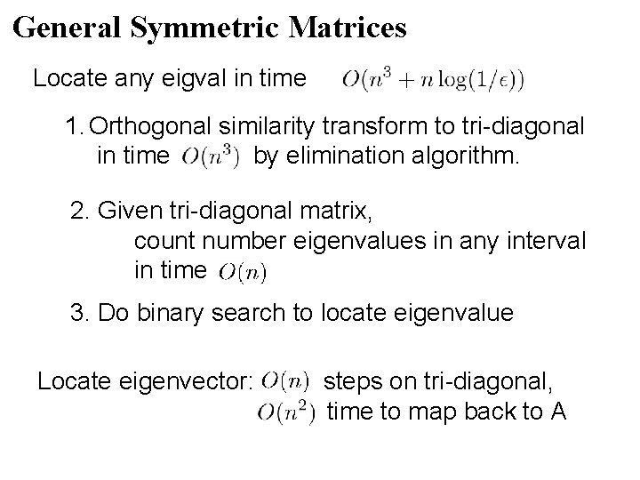
General Symmetric Matrices Locate any eigval in time 1. Orthogonal similarity transform to tri-diagonal in time by elimination algorithm. 2. Given tri-diagonal matrix, count number eigenvalues in any interval in time 3. Do binary search to locate eigenvalue Locate eigenvector: steps on tri-diagonal, time to map back to A

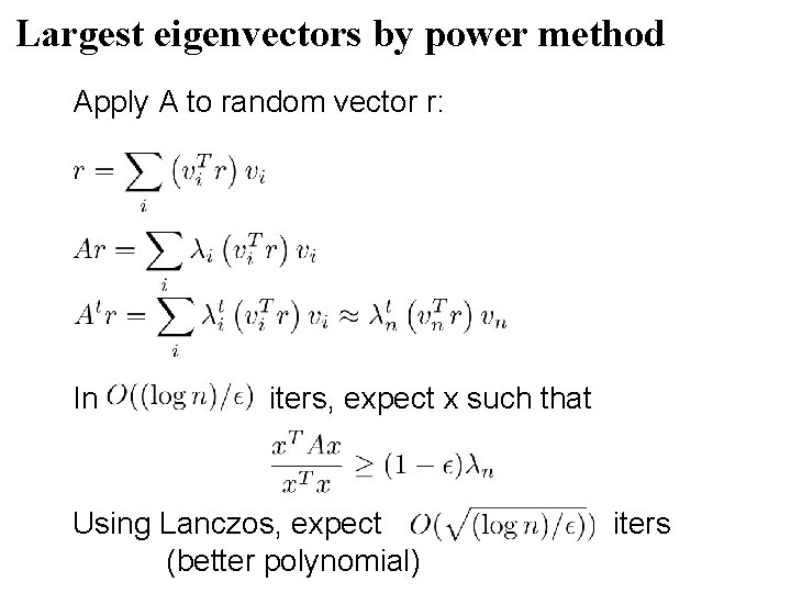
Largest eigenvectors by power method Apply A to random vector r: In iters, expect x such that Using Lanczos, expect (better polynomial) iters

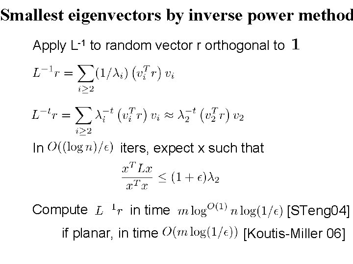
Smallest eigenvectors by inverse power method Apply L-1 to random vector r orthogonal to In iters, expect x such that Compute in time if planar, in time [STeng 04] [Koutis-Miller 06]

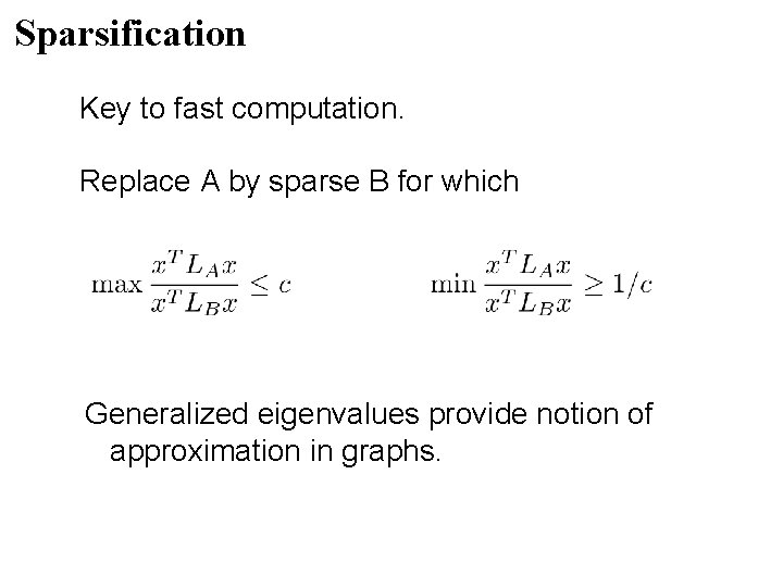
Sparsification Key to fast computation. Replace A by sparse B for which Generalized eigenvalues provide notion of approximation in graphs.

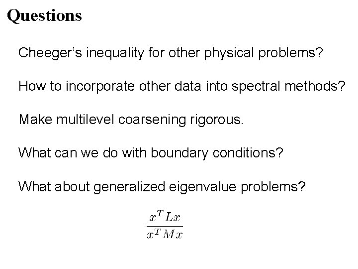
Questions Cheeger’s inequality for other physical problems? How to incorporate other data into spectral methods? Make multilevel coarsening rigorous. What can we do with boundary conditions? What about generalized eigenvalue problems?