ENGR 201 Statistics for Engineers Chapter 9 Test

ENGR 201: Statistics for Engineers Chapter 9: Test of Hypothesis for a Single Sample Null and alternative hypothesis, test statistic, type I and type II errors, significance level, p-value

Lecture Outline • What is Hypothesis Testing? • Hypothesis Formulation • Statistical Errors • Effect of Study Design • Test Procedures • Test Selection.

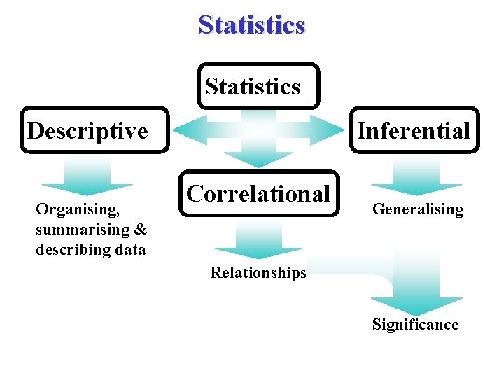
Statistics Descriptive Organising, summarising & describing data Inferential Correlational Generalising Relationships Significance

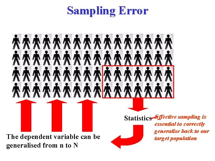
Sampling Error Statistics Effective sampling is The dependent variable can be generalised from n to N essential to correctly generalise back to our target population

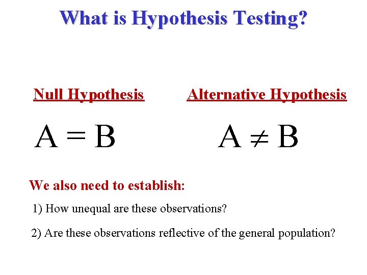
What is Hypothesis Testing? Null Hypothesis A=B Alternative Hypothesis A B We also need to establish: 1) How unequal are these observations? 2) Are these observations reflective of the general population?

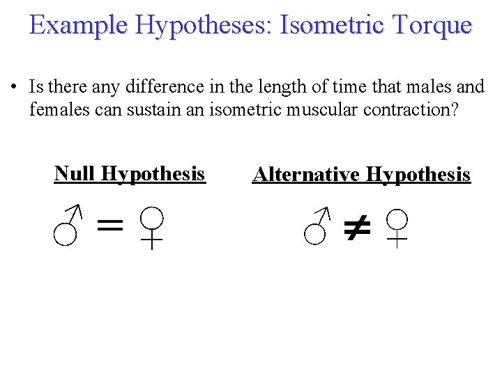
Example Hypotheses: Isometric Torque • Is there any difference in the length of time that males and females can sustain an isometric muscular contraction? Null Hypothesis ♂ = ♀ Alternative Hypothesis ♂ ♀

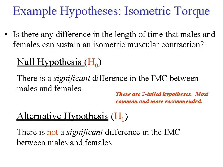
Example Hypotheses: Isometric Torque • Is there any difference in the length of time that males and females can sustain an isometric muscular contraction? Null Hypothesis (H 0) There is a significant difference in the IMC between males and females. These are 2 -tailed hypotheses. Most common and more recommended. Alternative Hypothesis (H 1) There is not a significant difference in the IMC between males and females

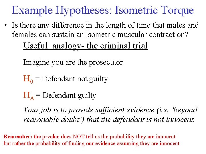
Example Hypotheses: Isometric Torque • Is there any difference in the length of time that males and females can sustain an isometric muscular contraction? Useful analogy- the criminal trial Imagine you are the prosecutor H 0 = Defendant not guilty HA = Defendant guilty Your job is to provide sufficient evidence (i. e. ‘beyond reasonable doubt’) that the defendant is not innocent. Remember: the p-value does NOT tell us the probability they are innocent but rather the probability of finding our evidence assuming they are innocent

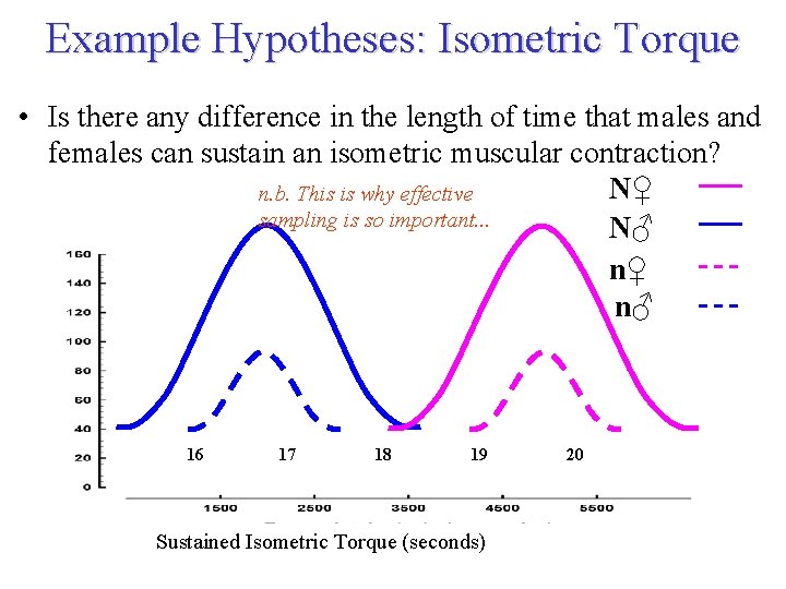
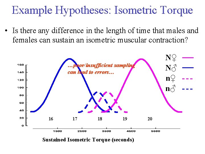
Example Hypotheses: Isometric Torque • Is there any difference in the length of time that males and females can sustain an isometric muscular contraction? N♀ n. b. This is why effective sampling is so important. . . N♂ n♀ n♂ 16 17 18 19 20 Sustained Isometric Torque (seconds)

Example Hypotheses: Isometric Torque • Is there any difference in the length of time that males and females can sustain an isometric muscular contraction? …poor/insufficient sampling can lead to errors… 16 17 18 19 20 Sustained Isometric Torque (seconds) N♀ N♂ n♀ n♂

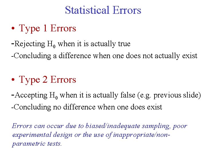
Statistical Errors • Type 1 Errors -Rejecting H 0 when it is actually true -Concluding a difference when one does not actually exist • Type 2 Errors -Accepting H 0 when it is actually false (e. g. previous slide) -Concluding no difference when one does exist Errors can occur due to biased/inadequate sampling, poor experimental design or the use of inappropriate/nonparametric tests.

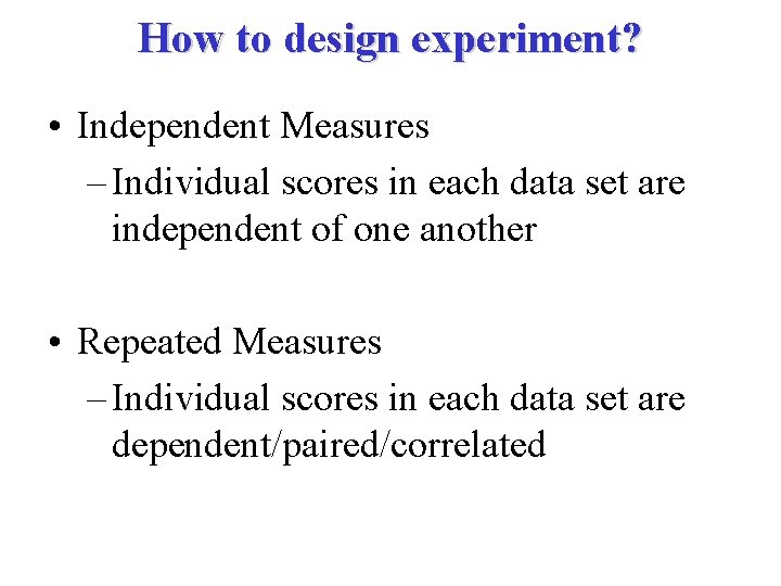
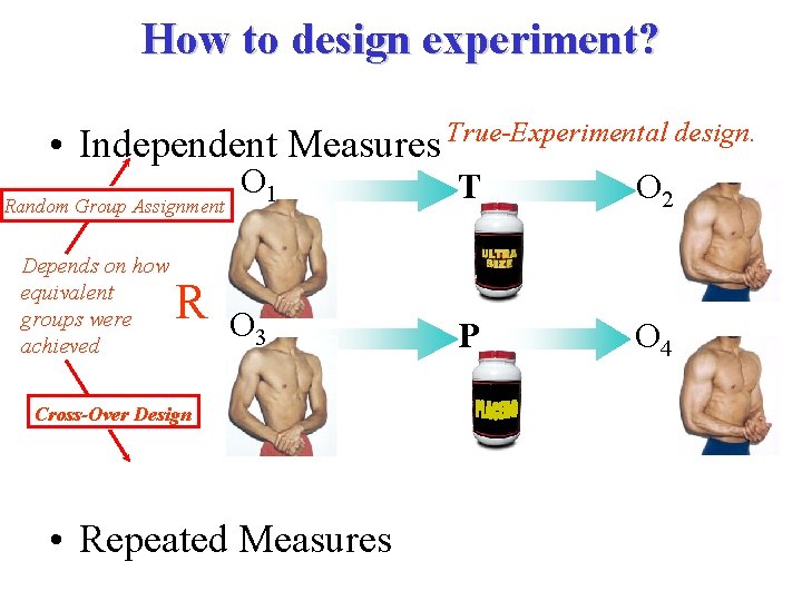
How to design experiment? • Independent Measures – Individual scores in each data set are independent of one another • Repeated Measures – Individual scores in each data set are dependent/paired/correlated

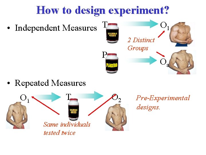
How to design experiment? • Independent Measures T O 1 Distinct – Individual scores in each 2 Groups data set are independent of one. Panother Oa • Repeated Measures Tscores in each O 2 data Pre-Experimental –OIndividual set are 1 dependent/paired/correlateddesigns. Same individuals tested twice

How to design experiment? True-Experimental design. • Independent Measures O 1 T O 2 Random Group Assignment – Individual scores in each data set are independent of one another Depends on how equivalent groups were achieved R O 3 Cross-Over Design • Repeated Measures P O 4

Testing: Introduction • Setting up and testing hypotheses is an essential part of statistical inference. In order to formulate such a test, usually some theory has been put forward, either because it is believed to be true or because it is to be used as a basis for argument, but has not been proved. • Hypothesis testing refers to the process of using statistical analysis to determine if the differences between observed and hypothesized values are due to random chance or to true differences in the samples. – Statistical tests separate significant effects from mere luck or random chance. – All hypothesis tests have unavoidable, but quantifiable, risks of making the wrong conclusion.

Testing: Introduction • Suppose that a pharmaceutical company is concerned that the mean potency of an antibiotic meet the minimum government potency standards. They need to decide between two possibilities: – The mean potency m does not exceed the required minimum potency. – The mean potency m exceeds the required minimum potency. • This is an example of a test of hypothesis.

Testing: Introduction • Similar to a courtroom trial. In trying a person for a crime, the jury needs to decide between one of two possibilities: – The person is guilty. – The person is innocent. • To begin with, the person is assumed innocent. • The prosecutor presents evidence, trying to convince the jury to reject the original assumption of innocence, and conclude that the person is guilty.

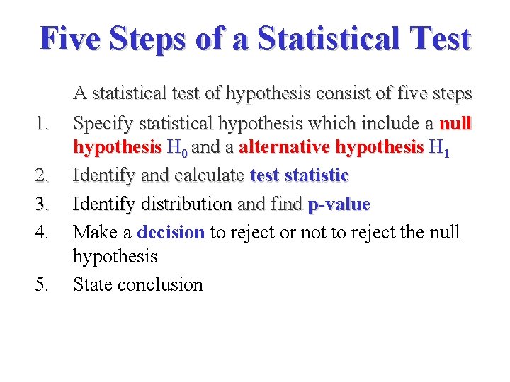
Five Steps of a Statistical Test A statistical test of hypothesis consist of five steps 1. 2. 3. 4. 5. Specify statistical hypothesis which include a null hypothesis H 0 and a alternative hypothesis H 1 Identify and calculate test statistic Identify distribution and find p-value Make a decision to reject or not to reject the null hypothesis State conclusion

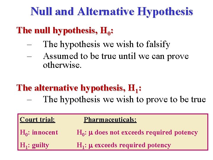
Null and Alternative Hypothesis The null hypothesis, H 0: – The hypothesis we wish to falsify – Assumed to be true until we can prove otherwise. The alternative hypothesis, H 1: – The hypothesis we wish to prove to be true Court trial: Pharmaceuticals: H 0: innocent H 0: m does not exceeds required potency H 1: guilty H 1: m exceeds required potency

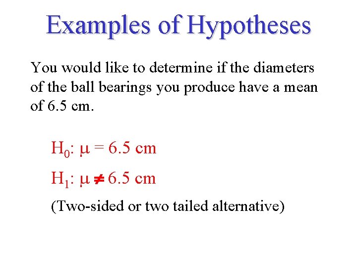
Examples of Hypotheses You would like to determine if the diameters of the ball bearings you produce have a mean of 6. 5 cm. H 0: = 6. 5 cm H 1: 6. 5 cm (Two-sided or two tailed alternative)

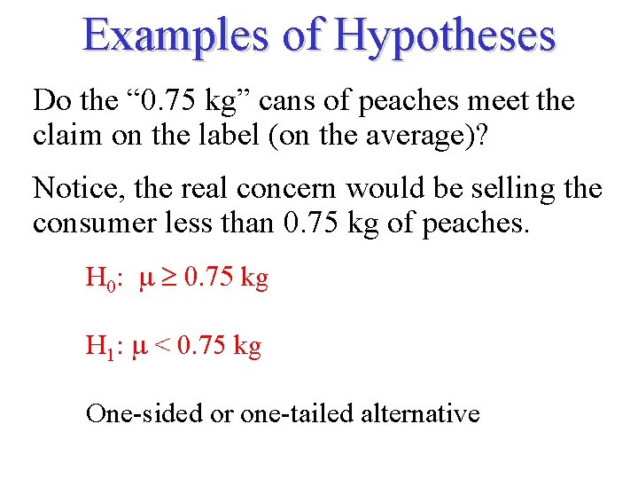
Examples of Hypotheses Do the “ 0. 75 kg” cans of peaches meet the claim on the label (on the average)? Notice, the real concern would be selling the consumer less than 0. 75 kg of peaches. H 0: 0. 75 kg H 1: < 0. 75 kg One-sided or one-tailed alternative

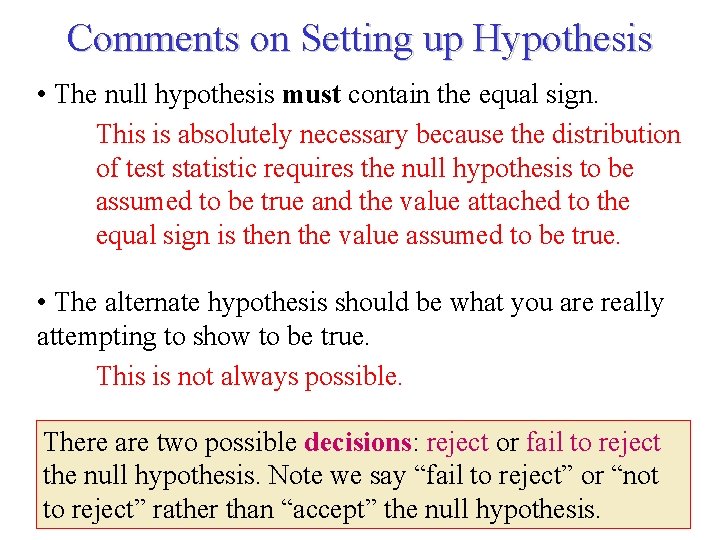
Comments on Setting up Hypothesis • The null hypothesis must contain the equal sign. This is absolutely necessary because the distribution of test statistic requires the null hypothesis to be assumed to be true and the value attached to the equal sign is then the value assumed to be true. • The alternate hypothesis should be what you are really attempting to show to be true. This is not always possible. There are two possible decisions: reject or fail to reject the null hypothesis. Note we say “fail to reject” or “not to reject” rather than “accept” the null hypothesis.

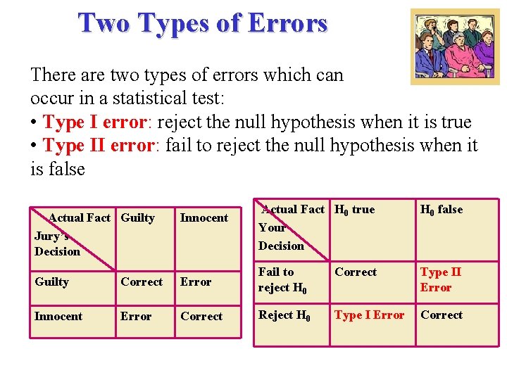
Two Types of Errors There are two types of errors which can occur in a statistical test: • Type I error: reject the null hypothesis when it is true • Type II error: fail to reject the null hypothesis when it is false Actual Fact H 0 true Your Decision H 0 false Error Fail to reject H 0 Correct Type II Error Correct Reject H 0 Type I Error Correct Actual Fact Guilty Jury’s Decision Innocent Guilty Correct Innocent Error

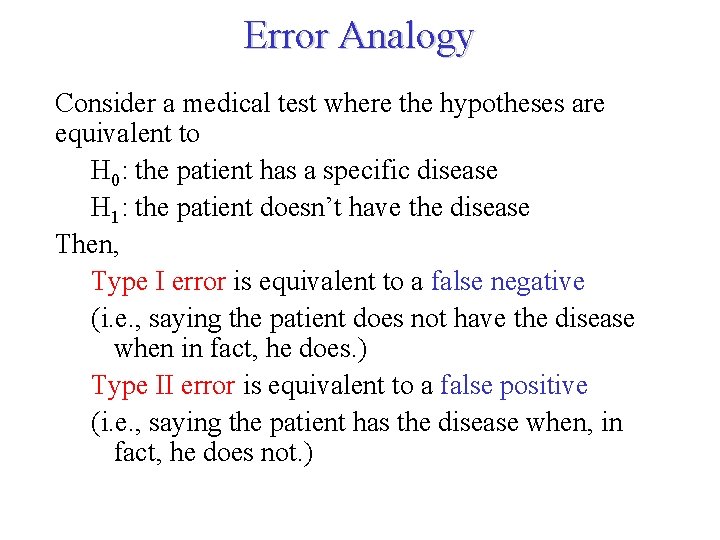
Error Analogy Consider a medical test where the hypotheses are equivalent to H 0: the patient has a specific disease H 1: the patient doesn’t have the disease Then, Type I error is equivalent to a false negative (i. e. , saying the patient does not have the disease when in fact, he does. ) Type II error is equivalent to a false positive (i. e. , saying the patient has the disease when, in fact, he does not. )

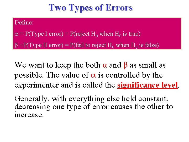
Two Types of Errors Define: = P(Type I error) = P(reject H 0 when H 0 is true) =P(Type II error) = P(fail to reject H 0 when H 0 is false) We want to keep the both α and β as small as possible. The value of is controlled by the experimenter and is called the significance level. Generally, with everything else held constant, decreasing one type of error causes the other to increase.

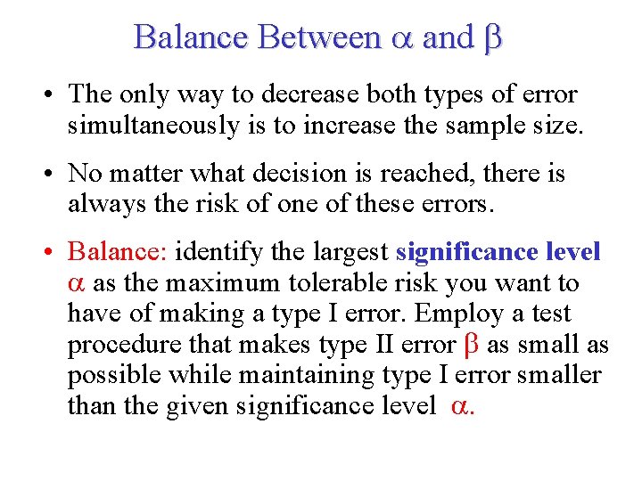
Balance Between and • The only way to decrease both types of error simultaneously is to increase the sample size. • No matter what decision is reached, there is always the risk of one of these errors. • Balance: identify the largest significance level as the maximum tolerable risk you want to have of making a type I error. Employ a test procedure that makes type II error as small as possible while maintaining type I error smaller than the given significance level .

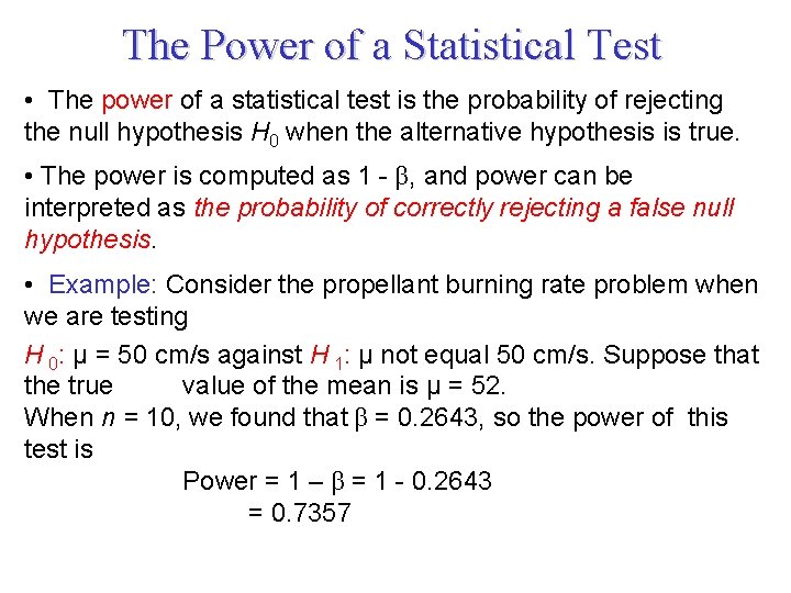
The Power of a Statistical Test • The power of a statistical test is the probability of rejecting the null hypothesis H 0 when the alternative hypothesis is true. • The power is computed as 1 - β, and power can be interpreted as the probability of correctly rejecting a false null hypothesis. • Example: Consider the propellant burning rate problem when we are testing H 0: μ = 50 cm/s against H 1: μ not equal 50 cm/s. Suppose that the true value of the mean is μ = 52. When n = 10, we found that β = 0. 2643, so the power of this test is Power = 1 – β = 1 - 0. 2643 = 0. 7357

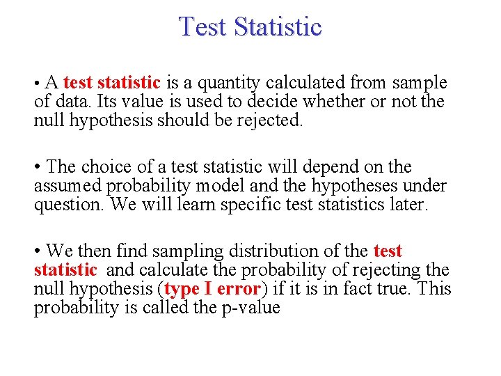
Test Statistic • A test statistic is a quantity calculated from sample of data. Its value is used to decide whether or not the null hypothesis should be rejected. • The choice of a test statistic will depend on the assumed probability model and the hypotheses under question. We will learn specific test statistics later. • We then find sampling distribution of the test statistic and calculate the probability of rejecting the null hypothesis (type I error) if it is in fact true. This probability is called the p-value

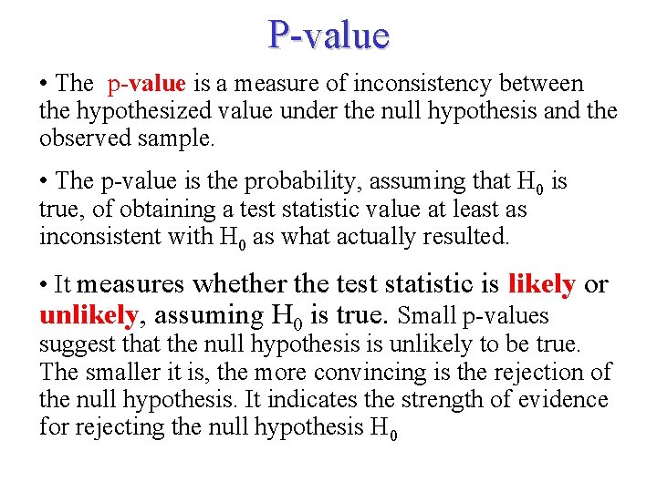
P-value • The p-value is a measure of inconsistency between the hypothesized value under the null hypothesis and the observed sample. • The p-value is the probability, assuming that H 0 is true, of obtaining a test statistic value at least as inconsistent with H 0 as what actually resulted. • It measures whether the test statistic is likely or unlikely, assuming H 0 is true. Small p-values suggest that the null hypothesis is unlikely to be true. The smaller it is, the more convincing is the rejection of the null hypothesis. It indicates the strength of evidence for rejecting the null hypothesis H 0

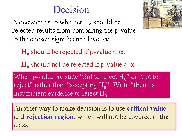
Decision A decision as to whether H 0 should be rejected results from comparing the p-value to the chosen significance level : – H 0 should be rejected if p-value . – H 0 should not be rejected if p-value > . When p-value>α, state “fail to reject H 0” or “not to reject” rather than “accepting H 0”. Write “there is insufficient evidence to reject H 0”. Another way to make decision is to use critical value and rejection region, which will not be covered in this class.

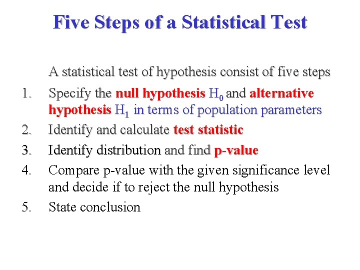
Five Steps of a Statistical Test A statistical test of hypothesis consist of five steps 1. 2. 3. 4. 5. Specify the null hypothesis H 0 and alternative hypothesis H 1 in terms of population parameters Identify and calculate test statistic Identify distribution and find p-value Compare p-value with the given significance level and decide if to reject the null hypothesis State conclusion

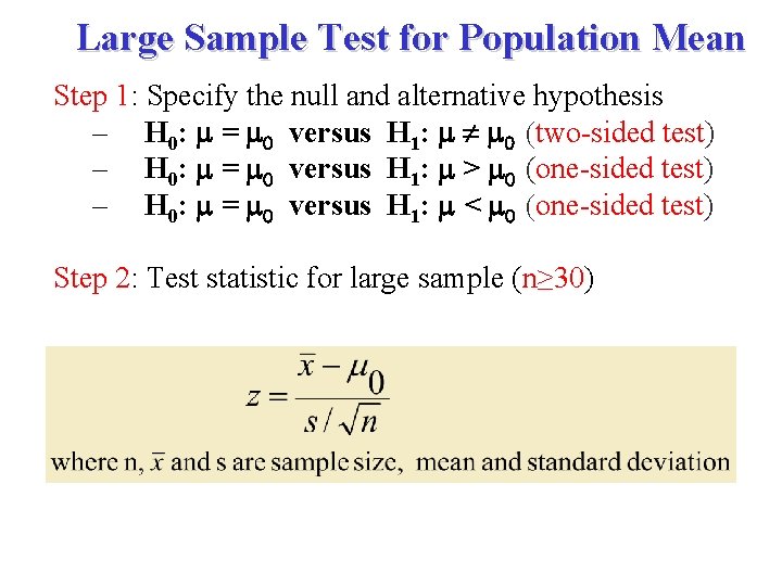
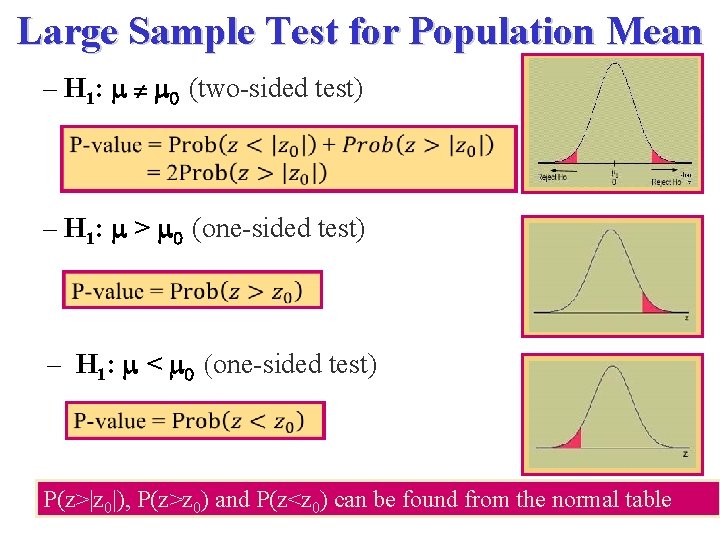
Large Sample Test for Population Mean Step 1: Specify the null and alternative hypothesis – H 0: m = m 0 versus H 1: m m 0 (two-sided test) – H 0: m = m 0 versus H 1: m > m 0 (one-sided test) – H 0: m = m 0 versus H 1: m < m 0 (one-sided test) Step 2: Test statistic for large sample (n≥ 30)

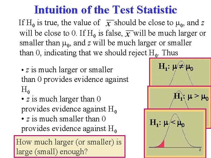
Intuition of the Test Statistic If H 0 is true, the value of should be close to 0, and z will be close to 0. If H 0 is false, will be much larger or smaller than 0, and z will be much larger or smaller than 0, indicating that we should reject H 0. Thus • z is much larger or smaller than 0 provides evidence against H 0 • z is much larger than 0 provides evidence against H 0 • z is much smaller than 0 provides evidence against H 0 How much larger (or smaller) is large (small) enough? H 1: m m 0 H 1: m > m 0 H 1: m < m 0

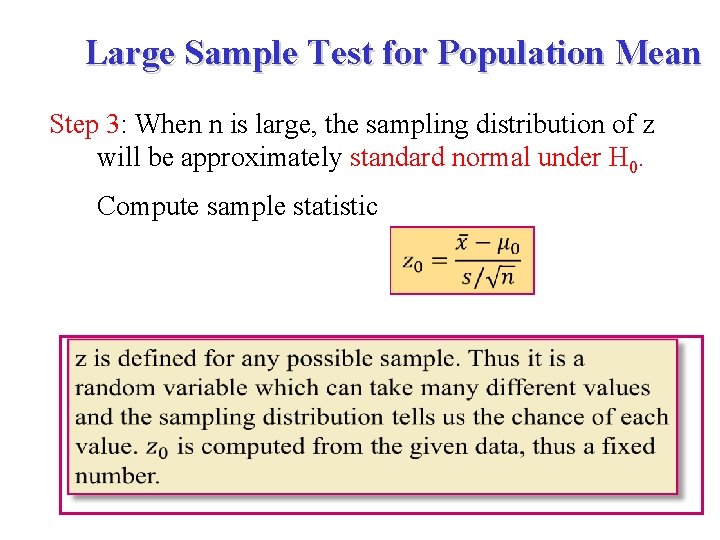
Large Sample Test for Population Mean Step 3: When n is large, the sampling distribution of z will be approximately standard normal under H 0. Compute sample statistic

Large Sample Test for Population Mean – H 1: m m 0 (two-sided test) – H 1: m > m 0 (one-sided test) – H 1: m < m 0 (one-sided test) P(z>|z 0|), P(z>z 0) and P(z<z 0) can be found from the normal table

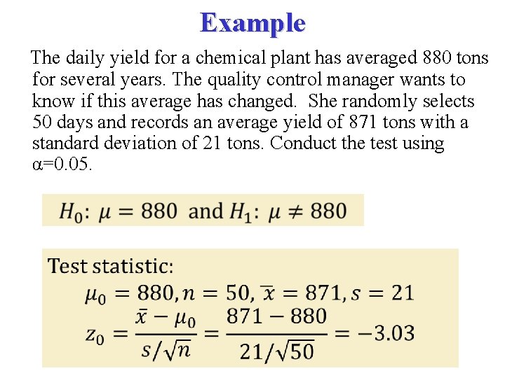
Example The daily yield for a chemical plant has averaged 880 tons for several years. The quality control manager wants to know if this average has changed. She randomly selects 50 days and records an average yield of 871 tons with a standard deviation of 21 tons. Conduct the test using α=0. 05.

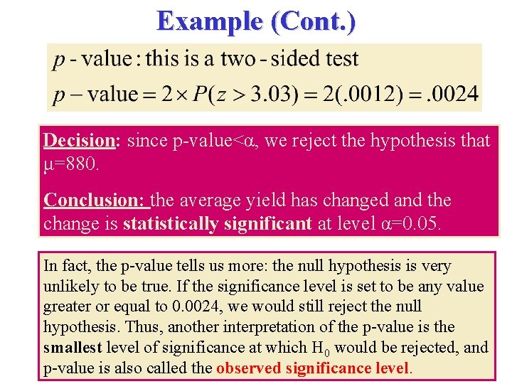
Example (Cont. ) Decision: since p-value<α, we reject the hypothesis that μ=880. Conclusion: the average yield has changed and the change is statistically significant at level α=0. 05. In fact, the p-value tells us more: the null hypothesis is very unlikely to be true. If the significance level is set to be any value greater or equal to 0. 0024, we would still reject the null hypothesis. Thus, another interpretation of the p-value is the smallest level of significance at which H 0 would be rejected, and p-value is also called the observed significance level.

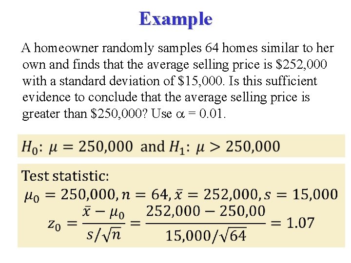
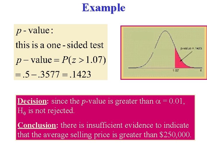
Example A homeowner randomly samples 64 homes similar to her own and finds that the average selling price is $252, 000 with a standard deviation of $15, 000. Is this sufficient evidence to conclude that the average selling price is greater than $250, 000? Use = 0. 01.

Example Decision: since the p-value is greater than = 0. 01, H 0 is not rejected. Conclusion: there is insufficient evidence to indicate that the average selling price is greater than $250, 000.

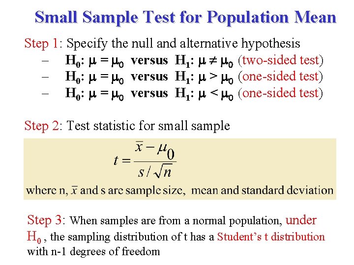
Small Sample Test for Population Mean Step 1: Specify the null and alternative hypothesis – H 0: m = m 0 versus H 1: m m 0 (two-sided test) – H 0: m = m 0 versus H 1: m > m 0 (one-sided test) – H 0: m = m 0 versus H 1: m < m 0 (one-sided test) Step 2: Test statistic for small sample Step 3: When samples are from a normal population, under H 0 , the sampling distribution of t has a Student’s t distribution with n-1 degrees of freedom

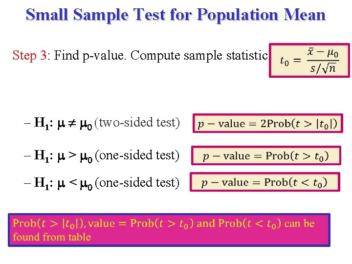
Small Sample Test for Population Mean Step 3: Find p-value. Compute sample statistic – H 1: m m 0 (two-sided test) – H 1: m > m 0 (one-sided test) – H 1: m < m 0 (one-sided test)

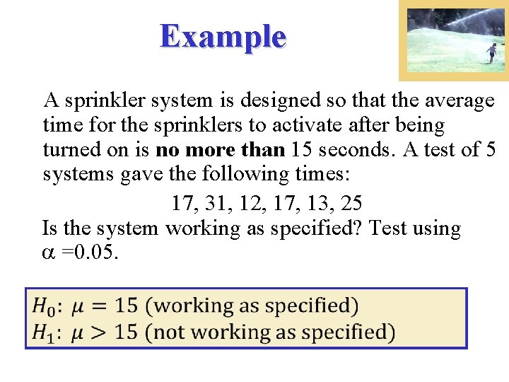
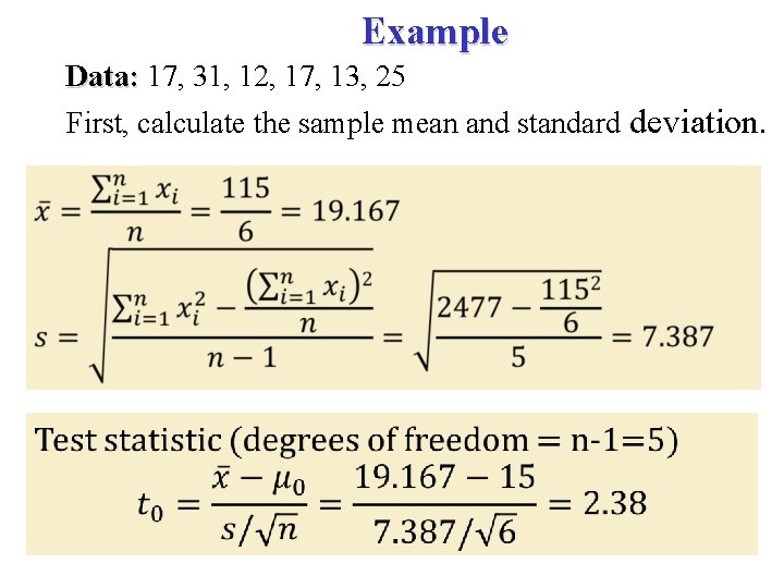
Example A sprinkler system is designed so that the average time for the sprinklers to activate after being turned on is no more than 15 seconds. A test of 5 systems gave the following times: 17, 31, 12, 17, 13, 25 Is the system working as specified? Test using =0. 05.

Example Data: 17, 31, 12, 17, 13, 25 First, calculate the sample mean and standard deviation.

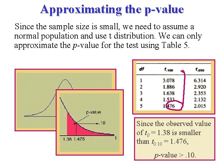
Approximating the p-value Since the sample size is small, we need to assume a normal population and use t distribution. We can only approximate the p-value for the test using Table 5. Since the observed value of t 0 = 1. 38 is smaller than t 0. 10 = 1. 476, p-value >. 10.

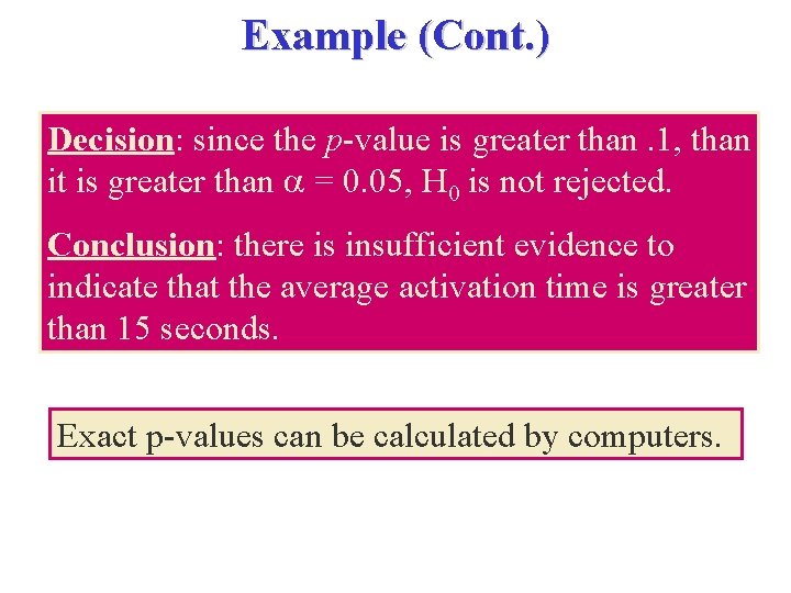
Example (Cont. ) Decision: since the p-value is greater than. 1, than it is greater than = 0. 05, H 0 is not rejected. Conclusion: there is insufficient evidence to indicate that the average activation time is greater than 15 seconds. Exact p-values can be calculated by computers.

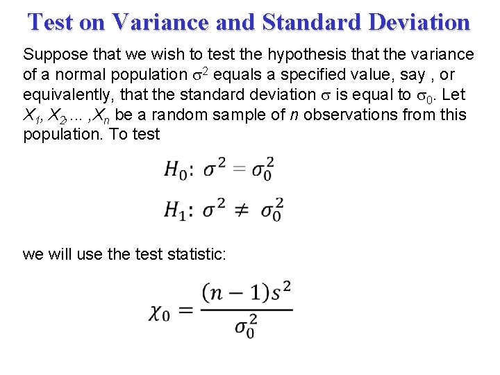
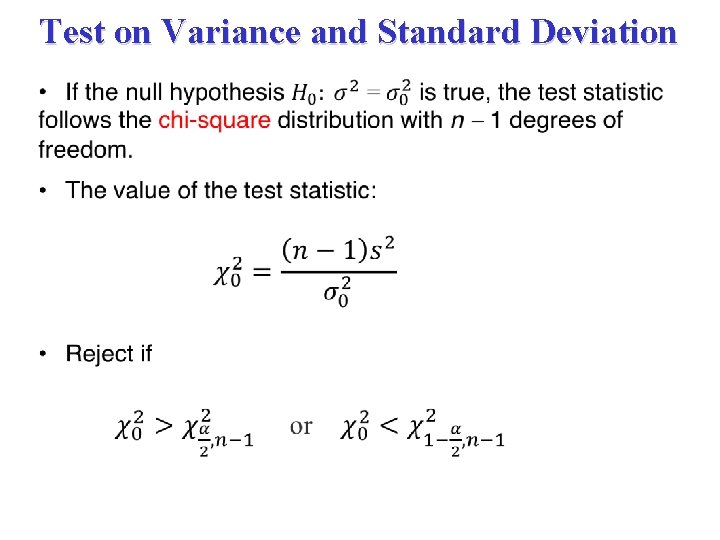
Test on Variance and Standard Deviation Suppose that we wish to test the hypothesis that the variance of a normal population 2 equals a specified value, say , or equivalently, that the standard deviation is equal to 0. Let X 1, X 2, . . . , Xn be a random sample of n observations from this population. To test we will use the test statistic:

Test on Variance and Standard Deviation

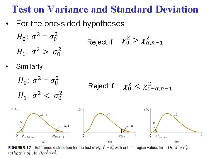
Test on Variance and Standard Deviation • For the one-sided hypotheses • Reject if Similarly Reject if

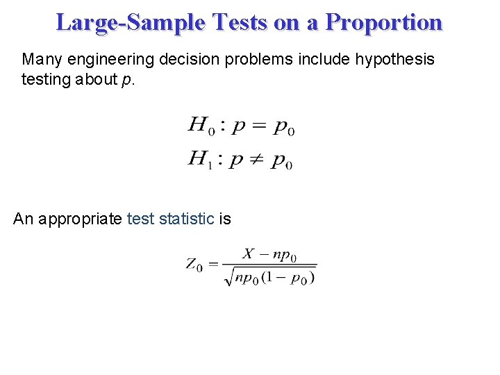
Large-Sample Tests on a Proportion Many engineering decision problems include hypothesis testing about p. An appropriate test statistic is

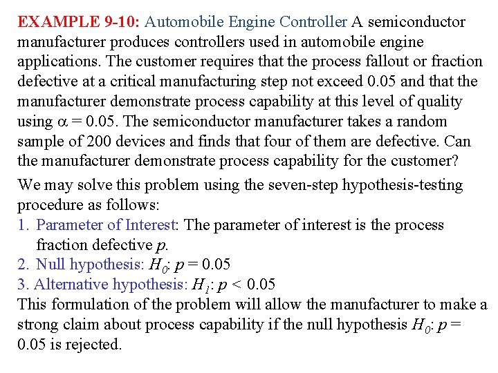
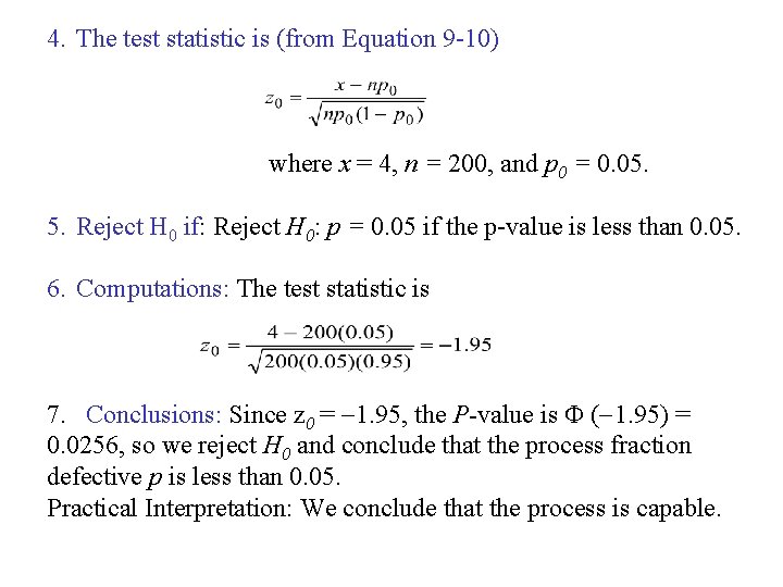
EXAMPLE 9 -10: Automobile Engine Controller A semiconductor manufacturer produces controllers used in automobile engine applications. The customer requires that the process fallout or fraction defective at a critical manufacturing step not exceed 0. 05 and that the manufacturer demonstrate process capability at this level of quality using = 0. 05. The semiconductor manufacturer takes a random sample of 200 devices and finds that four of them are defective. Can the manufacturer demonstrate process capability for the customer? We may solve this problem using the seven-step hypothesis-testing procedure as follows: 1. Parameter of Interest: The parameter of interest is the process fraction defective p. 2. Null hypothesis: H 0: p = 0. 05 3. Alternative hypothesis: H 1: p < 0. 05 This formulation of the problem will allow the manufacturer to make a strong claim about process capability if the null hypothesis H 0: p = 0. 05 is rejected.

4. The test statistic is (from Equation 9 -10) where x = 4, n = 200, and p 0 = 0. 05. 5. Reject H 0 if: Reject H 0: p = 0. 05 if the p-value is less than 0. 05. 6. Computations: The test statistic is 7. Conclusions: Since z 0 = 1. 95, the P-value is ( 1. 95) = 0. 0256, so we reject H 0 and conclude that the process fraction defective p is less than 0. 05. Practical Interpretation: We conclude that the process is capable.

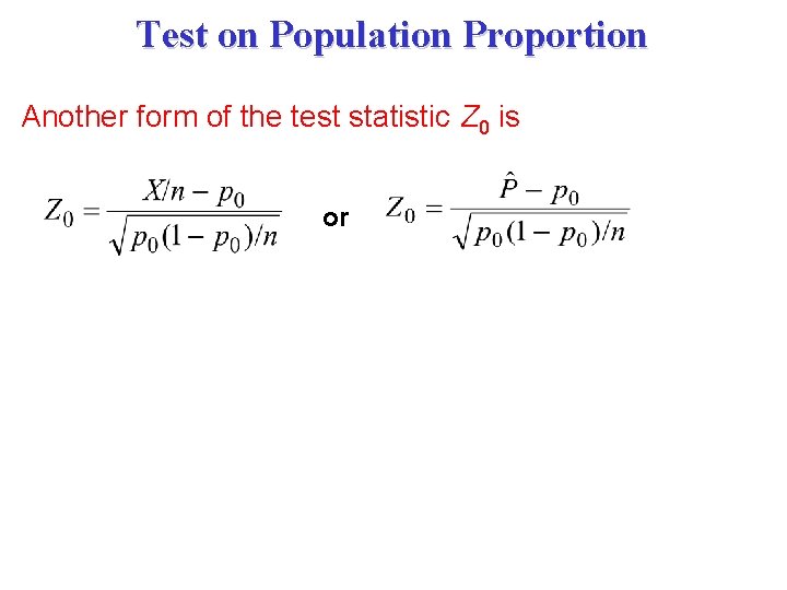
Test on Population Proportion Another form of the test statistic Z 0 is or

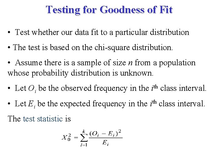
Testing for Goodness of Fit • Test whether our data fit to a particular distribution • The test is based on the chi-square distribution. • Assume there is a sample of size n from a population whose probability distribution is unknown. • Let Oi be the observed frequency in the ith class interval. • Let Ei be the expected frequency in the ith class interval. The test statistic is

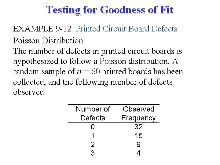
Testing for Goodness of Fit EXAMPLE 9 -12 Printed Circuit Board Defects Poisson Distribution The number of defects in printed circuit boards is hypothesized to follow a Poisson distribution. A random sample of n = 60 printed boards has been collected, and the following number of defects observed. Number of Defects 0 1 2 3 Observed Frequency 32 15 9 4

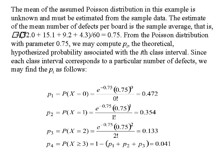
The mean of the assumed Poisson distribution in this example is unknown and must be estimated from the sample data. The estimate of the mean number of defects per board is the sample average, that is, �� =(32. 0 + 15. 1 + 9. 2 + 4. 3)/60 = 0. 75. From the Poisson distribution with parameter 0. 75, we may compute pi, theoretical, hypothesized probability associated with the ith class interval. Since each class interval corresponds to a particular number of defects, we may find the pi as follows:

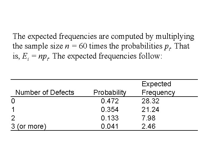
The expected frequencies are computed by multiplying the sample size n = 60 times the probabilities pi. That is, Ei = npi. The expected frequencies follow: Number of Defects 0 1 2 3 (or more) Probability 0. 472 0. 354 0. 133 0. 041 Expected Frequency 28. 32 21. 24 7. 98 2. 46

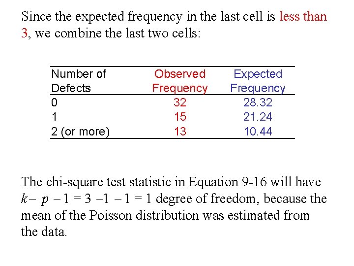
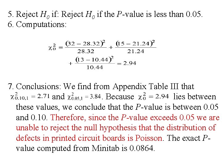
Since the expected frequency in the last cell is less than 3, we combine the last two cells: Number of Defects 0 1 2 (or more) Observed Frequency 32 15 13 Expected Frequency 28. 32 21. 24 10. 44 The chi-square test statistic in Equation 9 -16 will have k p 1 = 3 1 1 = 1 degree of freedom, because the mean of the Poisson distribution was estimated from the data.

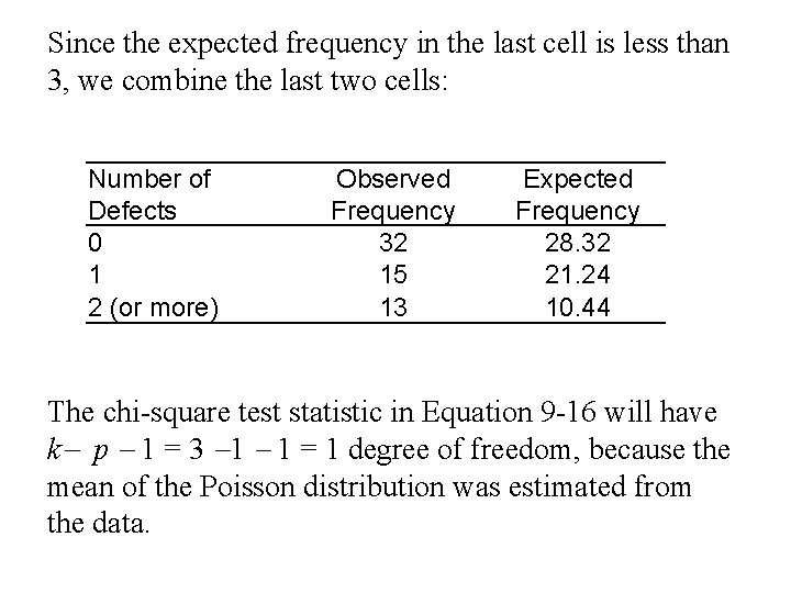
Since the expected frequency in the last cell is less than 3, we combine the last two cells: Number of Defects 0 1 2 (or more) Observed Frequency 32 15 13 Expected Frequency 28. 32 21. 24 10. 44 The chi-square test statistic in Equation 9 -16 will have k p 1 = 3 1 1 = 1 degree of freedom, because the mean of the Poisson distribution was estimated from the data.

5. Reject H 0 if: Reject H 0 if the P-value is less than 0. 05. 6. Computations: 7. Conclusions: We find from Appendix Table III that and. Because lies between these values, we conclude that the P-value is between 0. 05 and 0. 10. Therefore, since the P-value exceeds 0. 05 we are unable to reject the null hypothesis that the distribution of defects in printed circuit boards is Poisson. The exact Pvalue computed from Minitab is 0. 0864.