ENGR 201 Statistics for Engineers Chapter 10 Statistical

ENGR 201: Statistics for Engineers Chapter 10: Statistical Inference for Two Samples - Inference on difference in means of two normal distribution A non-parametric test on the differences in two means Paired t-test Inference on variances, population proportions

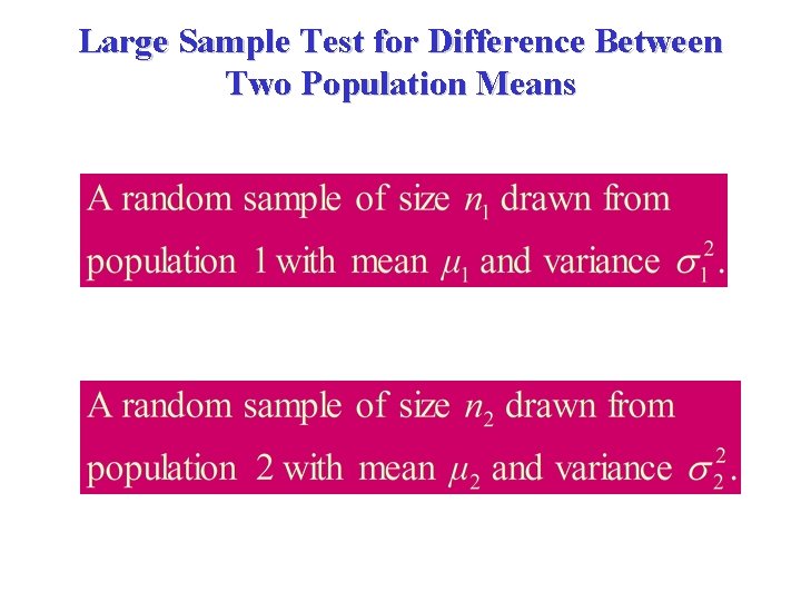
Large Sample Test for Difference Between Two Population Means

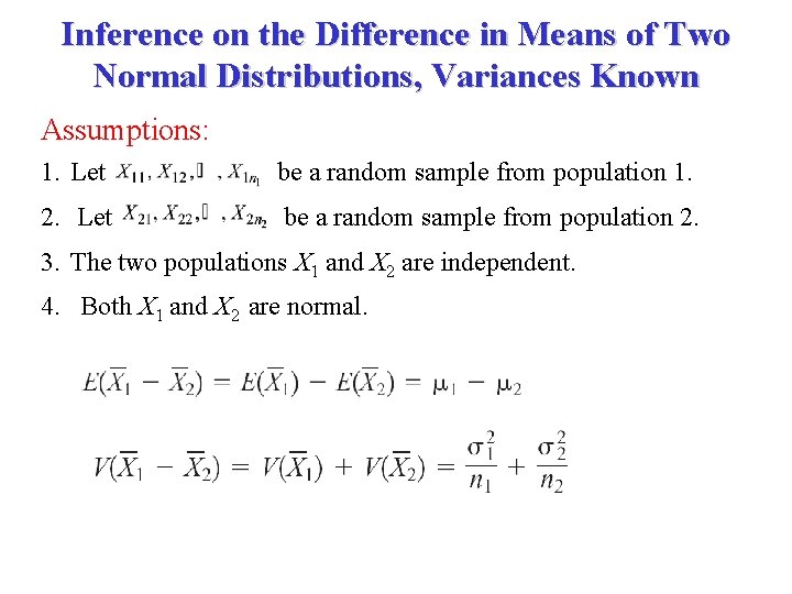
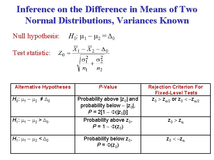
Inference on the Difference in Means of Two Normal Distributions, Variances Known Assumptions: 1. Let be a random sample from population 1. 2. Let be a random sample from population 2. 3. The two populations X 1 and X 2 are independent. 4. Both X 1 and X 2 are normal.

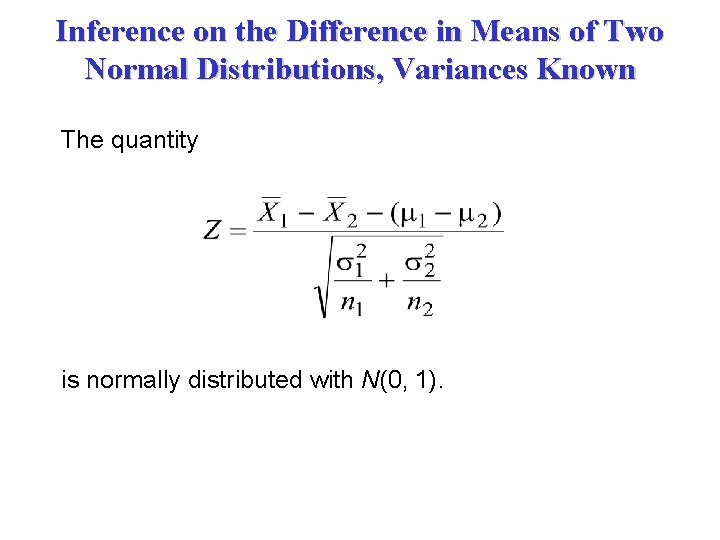
Inference on the Difference in Means of Two Normal Distributions, Variances Known The quantity is normally distributed with N(0, 1).

Inference on the Difference in Means of Two Normal Distributions, Variances Known Null hypothesis: H 0: 1 2 = 0 Test statistic: Alternative Hypotheses P-Value Rejection Criterion For Fixed-Level Tests H 0 : 1 2 ≠ 0 Probability above |z 0| and probability below |z 0|, P = 2[1 (|z 0|)] z 0 z 2 or z 0 z 2 H 1 : 1 2 > 0 Probability above z 0, P = 1 (z 0) z 0 z H 1 : 1 2 < 0 Probability below z 0, P = (z 0) z 0 z

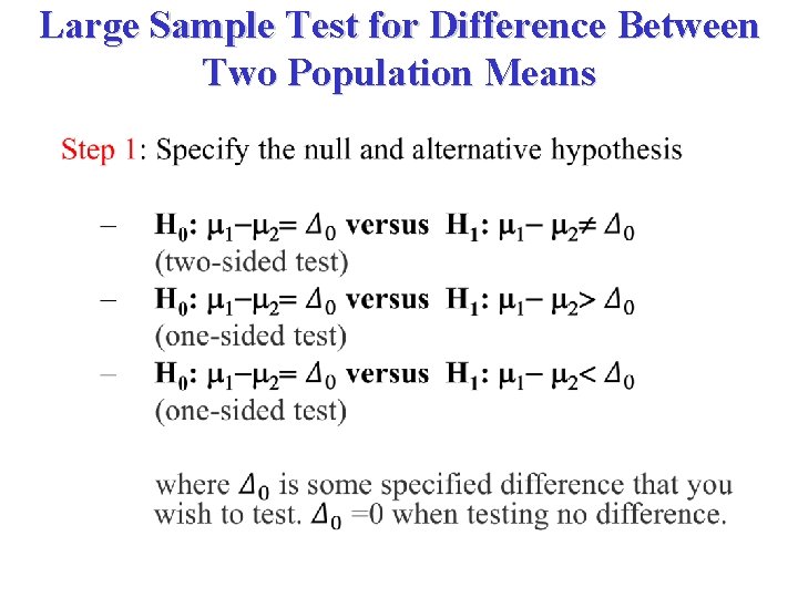
Large Sample Test for Difference Between Two Population Means •

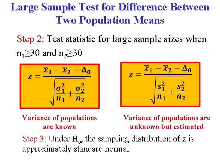
Large Sample Test for Difference Between Two Population Means Step 2: Test statistic for large sample sizes when n 1≥ 30 and n 2≥ 30 Variance of populations are known Variance of populations are unknown but estimated Step 3: Under H 0, the sampling distribution of z is approximately standard normal

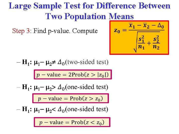
Large Sample Test for Difference Between Two Population Means Step 3: Find p-value. Compute

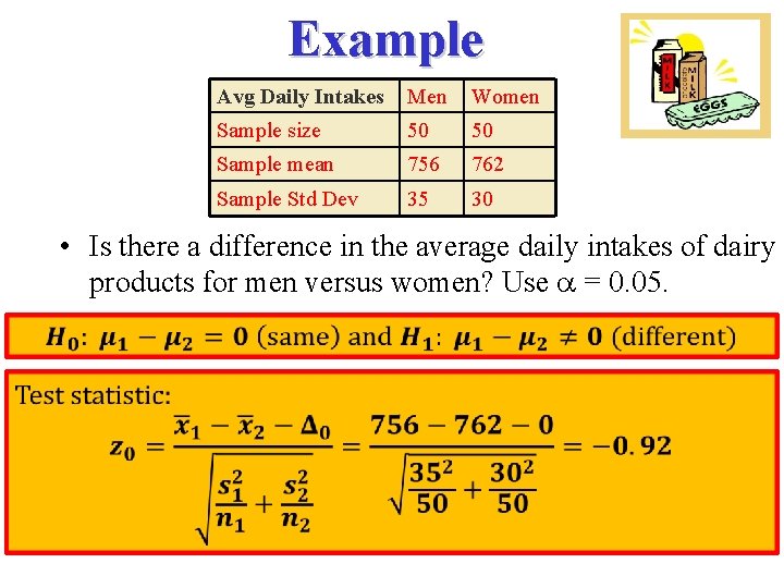
Example Avg Daily Intakes Men Women Sample size 50 50 Sample mean 756 762 Sample Std Dev 35 30 • Is there a difference in the average daily intakes of dairy products for men versus women? Use = 0. 05.

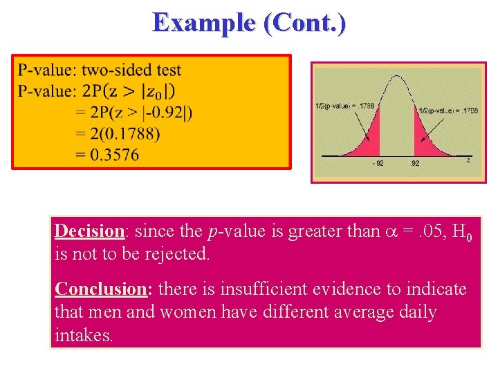
Example (Cont. ) Decision: since the p-value is greater than =. 05, H 0 is not to be rejected. Conclusion: there is insufficient evidence to indicate that men and women have different average daily intakes.

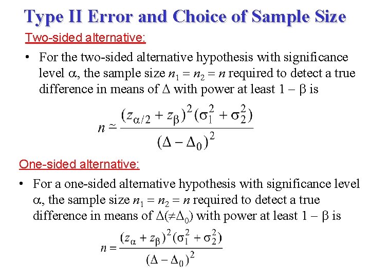
Type II Error and Choice of Sample Size Two-sided alternative: • For the two-sided alternative hypothesis with significance level , the sample size n 1 n 2 n required to detect a true difference in means of with power at least 1 is One-sided alternative: • For a one-sided alternative hypothesis with significance level , the sample size n 1 n 2 n required to detect a true difference in means of ( 0) with power at least 1 is

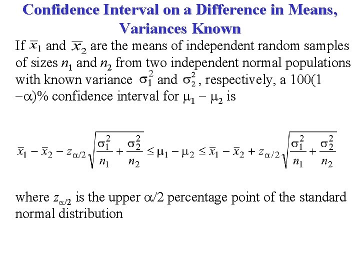
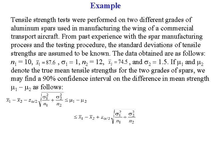
Confidence Interval on a Difference in Means, Variances Known If and are the means of independent random samples of sizes n 1 and n 2 from two independent normal populations with known variance and , respectively, a 100(1 ) confidence interval for 1 2 is where z 2 is the upper 2 percentage point of the standard normal distribution

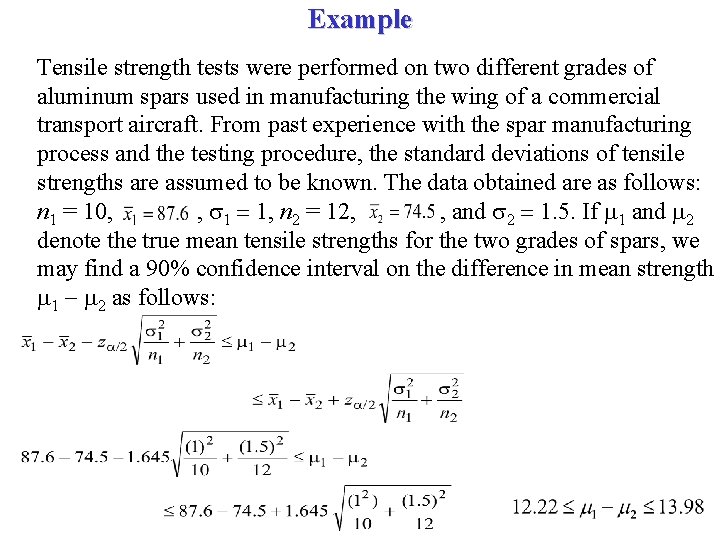
Example Tensile strength tests were performed on two different grades of aluminum spars used in manufacturing the wing of a commercial transport aircraft. From past experience with the spar manufacturing process and the testing procedure, the standard deviations of tensile strengths are assumed to be known. The data obtained are as follows: n 1 = 10, , 1 1, n 2 = 12, , and 2 1. 5. If 1 and 2 denote the true mean tensile strengths for the two grades of spars, we may find a 90% confidence interval on the difference in mean strength 1 2 as follows:

Example Tensile strength tests were performed on two different grades of aluminum spars used in manufacturing the wing of a commercial transport aircraft. From past experience with the spar manufacturing process and the testing procedure, the standard deviations of tensile strengths are assumed to be known. The data obtained are as follows: n 1 = 10, , 1 1, n 2 = 12, , and 2 1. 5. If 1 and 2 denote the true mean tensile strengths for the two grades of spars, we may find a 90% confidence interval on the difference in mean strength 1 2 as follows:

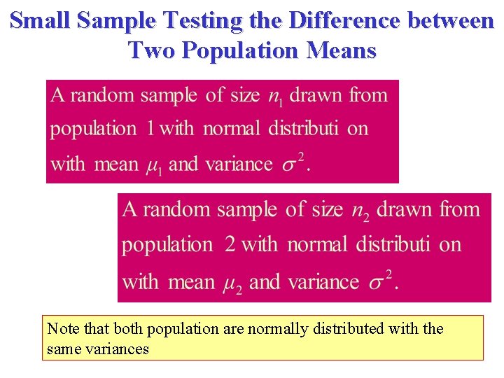
Small Sample Testing the Difference between Two Population Means Note that both population are normally distributed with the same variances

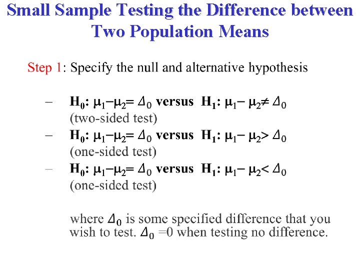
Small Sample Testing the Difference between Two Population Means •

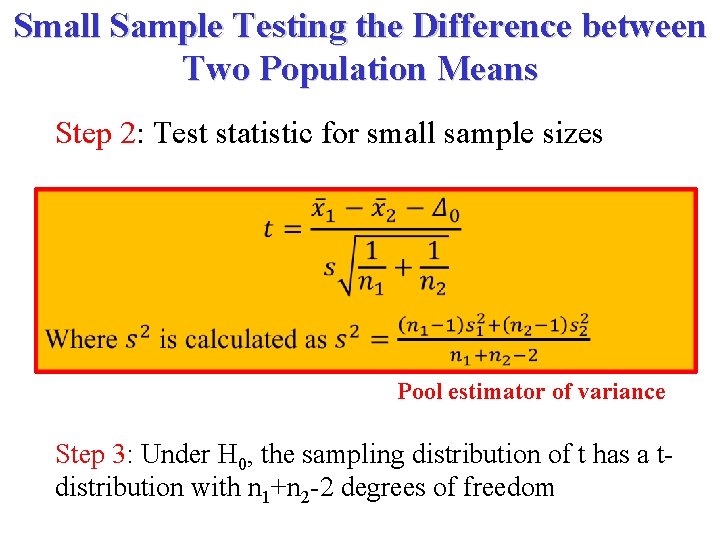
Small Sample Testing the Difference between Two Population Means Step 2: Test statistic for small sample sizes Pool estimator of variance Step 3: Under H 0, the sampling distribution of t has a t- distribution with n 1+n 2 -2 degrees of freedom

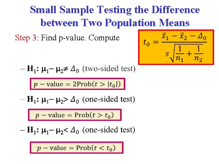
Small Sample Testing the Difference between Two Population Means Step 3: Find p-value. Compute

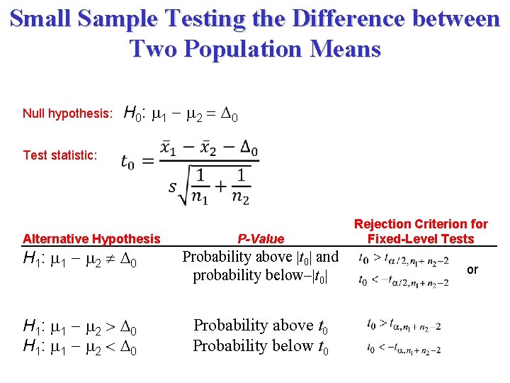
Small Sample Testing the Difference between Two Population Means Null hypothesis: Test statistic: H 0: 1 2 0 Alternative Hypothesis P-Value H 1: 1 2 0 Probability above t 0 and probability below t 0 H 1: 1 2 0 Probability above t 0 Probability below t 0 Rejection Criterion for Fixed-Level Tests or

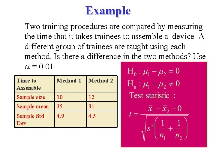
Example Two training procedures are compared by measuring the time that it takes trainees to assemble a device. A different group of trainees are taught using each method. Is there a difference in the two methods? Use = 0. 01. Time to Assemble Method 1 Method 2 Sample size 10 12 Sample mean 35 31 Sample Std Dev 4. 9 4. 5

Example (Cont. ) Time to Assemble Method 1 Method 2 Sample size 10 12 Sample mean 35 31 Sample Std Dev 4. 9 4. 5

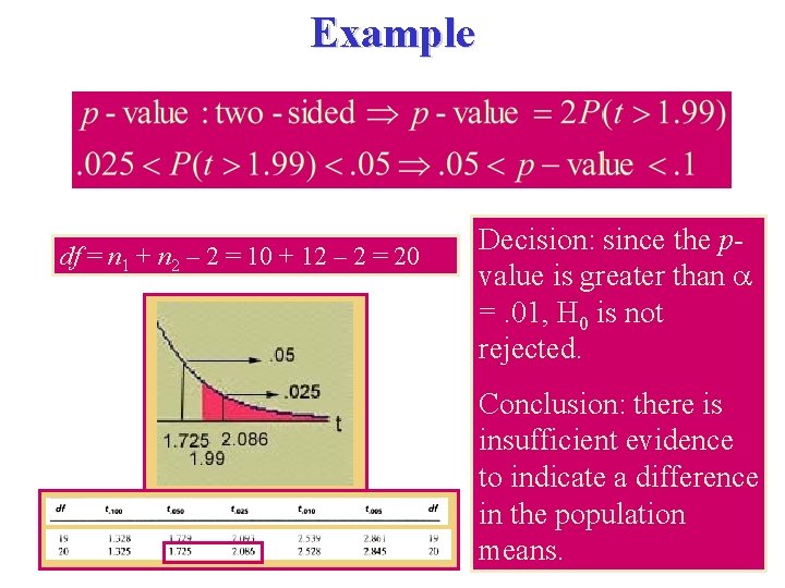
Example df = n 1 + n 2 – 2 = 10 + 12 – 2 = 20 Decision: since the pvalue is greater than =. 01, H 0 is not rejected. Conclusion: there is insufficient evidence to indicate a difference in the population means.

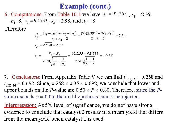
Example Two catalysts are being analyzed to determine how they affect the mean yield of a chemical process. Specifically, catalyst 1 is currently in use, but catalyst 2 is acceptable. Since catalyst 2 is cheaper, it should be adopted, providing it does not change the process yield. A test is run in the pilot plant and results in the data shown in Table 101. Is there any difference between the mean yields? Use 0. 05, and assume equal variances. Observation Number Catalyst 1 Catalyst 2 1 2 3 4 5 6 7 8 91. 50 94. 18 92. 18 95. 39 91. 79 89. 07 94. 72 89. 21 89. 19 90. 95 90. 46 93. 21 97. 19 97. 04 91. 07 92. 75 2. 39 ss 11 = 2. 39 ss 2 =2. 98 2

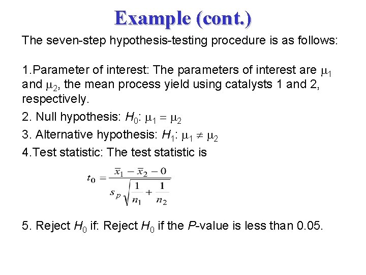
Example (cont. ) The seven-step hypothesis-testing procedure is as follows: 1. Parameter of interest: The parameters of interest are 1 and 2, the mean process yield using catalysts 1 and 2, respectively. 2. Null hypothesis: H 0: 1 2 3. Alternative hypothesis: H 1: 1 2 4. Test statistic: The test statistic is 5. Reject H 0 if: Reject H 0 if the P-value is less than 0. 05.

Example (cont. ) 6. Computations: From Table 10 -1 we have , s 1 = 2. 39, n 1=8, , s 2 = 2. 98, and n 2 = 8. Therefore 7. Conclusions: From Appendix Table V we can find t 0. 40, 14 0. 258 and t 0. 25, 14 0. 692. Since, 0. 258 0. 35 0. 692, we conclude that lower and upper bounds on the P-value are 0. 50 P 0. 80. Therefore, since the Pvalue exceeds 0. 05, the null hypothesis cannot be rejected. Interpretation: At 5% level of significance, we do not have strong evidence to conclude that catalyst 2 results in a mean yield that differs from the mean yield when catalyst 1 is used.

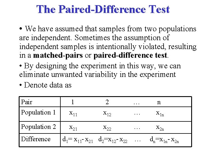
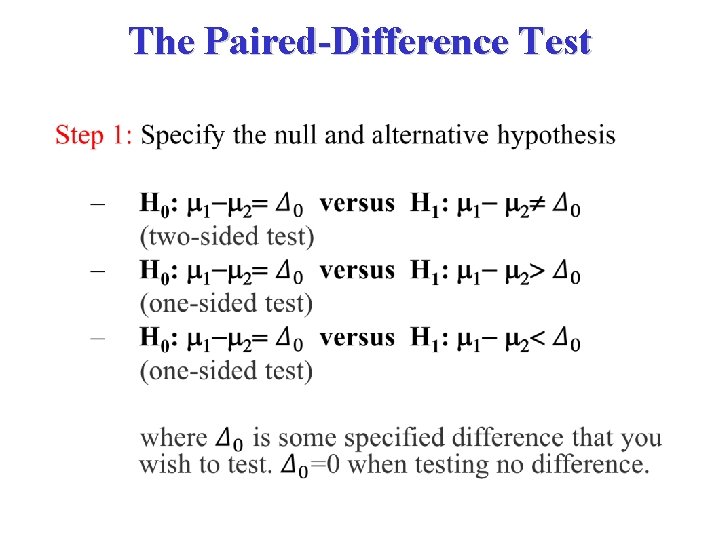
The Paired-Difference Test • We have assumed that samples from two populations are independent. Sometimes the assumption of independent samples is intentionally violated, resulting in a matched-pairs or matched-pairs paired-difference test • By designing the experiment in this way, we can eliminate unwanted variability in the experiment • Denote data as Pair 1 2 … n Population 1 x 11 x 12 … x 1 n Population 2 x 21 x 22 … x 2 n Difference d 1= x 11 - x 21 d 2=x 12 - x 22 … dn=x 1 n- x 2 n

The Paired-Difference Test •

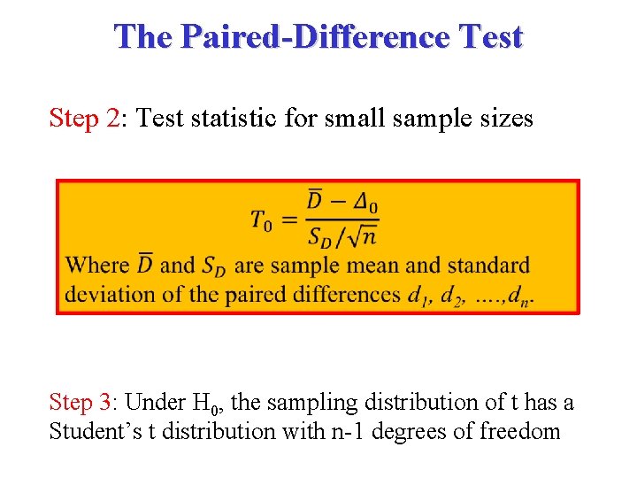
The Paired-Difference Test Step 2: Test statistic for small sample sizes Step 3: Under H 0, the sampling distribution of t has a Student’s t distribution with n-1 degrees of freedom

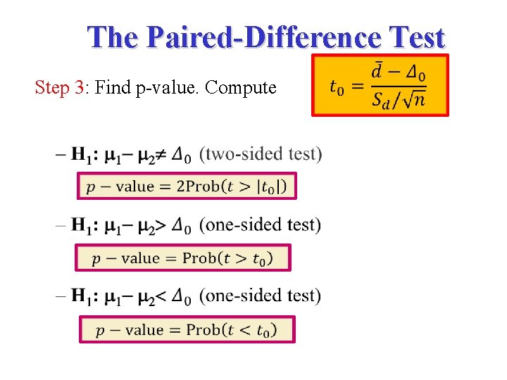
The Paired-Difference Test Step 3: Find p-value. Compute

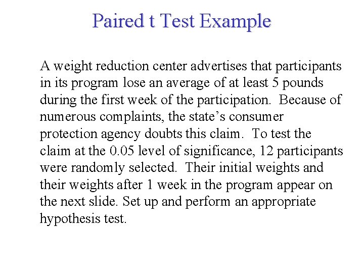
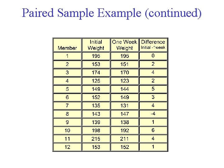
Paired t Test Example A weight reduction center advertises that participants in its program lose an average of at least 5 pounds during the first week of the participation. Because of numerous complaints, the state’s consumer protection agency doubts this claim. To test the claim at the 0. 05 level of significance, 12 participants were randomly selected. Their initial weights and their weights after 1 week in the program appear on the next slide. Set up and perform an appropriate hypothesis test.

Paired Sample Example (continued)

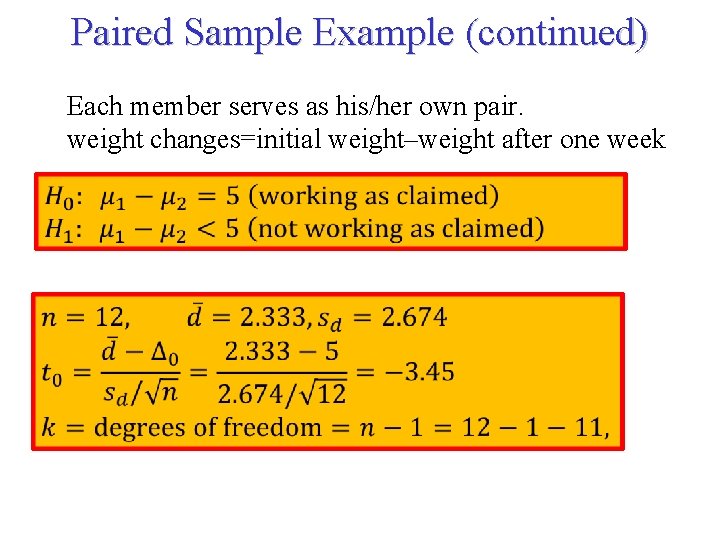
Paired Sample Example (continued) Each member serves as his/her own pair. weight changes=initial weight–weight after one week

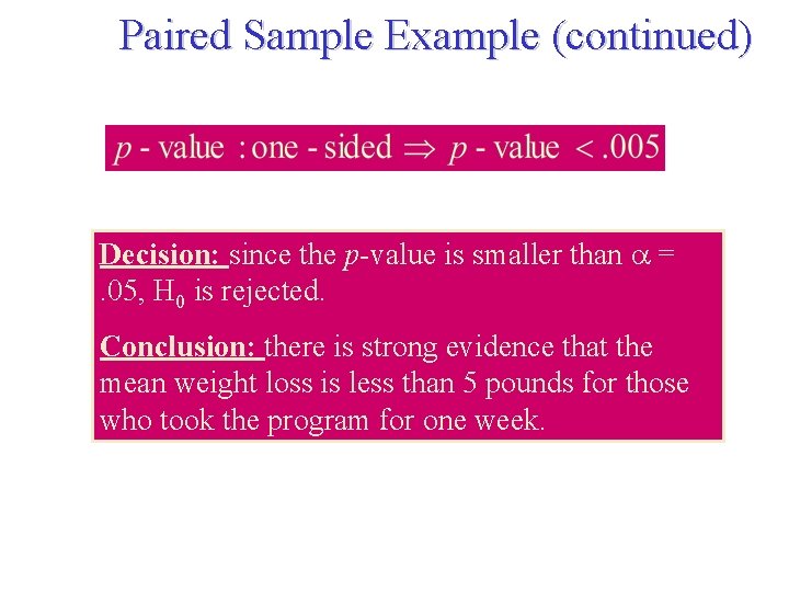
Paired Sample Example (continued) Decision: since the p-value is smaller than = . 05, H 0 is rejected. Conclusion: there is strong evidence that the mean weight loss is less than 5 pounds for those who took the program for one week.

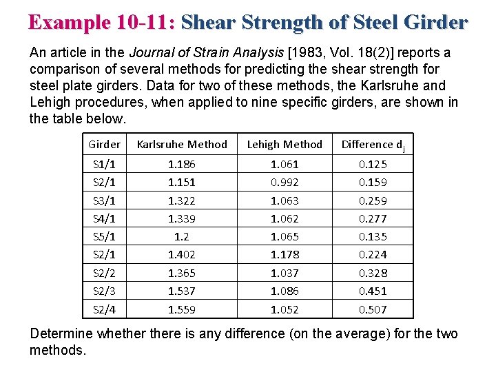
Example 10 -11: Shear Strength of Steel Girder An article in the Journal of Strain Analysis [1983, Vol. 18(2)] reports a comparison of several methods for predicting the shear strength for steel plate girders. Data for two of these methods, the Karlsruhe and Lehigh procedures, when applied to nine specific girders, are shown in the table below. Girder Karlsruhe Method Lehigh Method Difference dj S 1/1 S 2/1 S 3/1 S 4/1 S 5/1 S 2/2 S 2/3 S 2/4 1. 186 1. 151 1. 322 1. 339 1. 2 1. 402 1. 365 1. 537 1. 559 1. 061 0. 992 1. 063 1. 062 1. 065 1. 178 1. 037 1. 086 1. 052 0. 125 0. 159 0. 277 0. 135 0. 224 0. 328 0. 451 0. 507 Determine whethere is any difference (on the average) for the two methods.

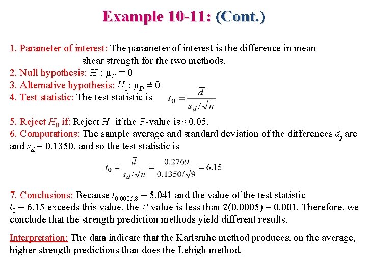
Example 10 -11: (Cont. ) 1. Parameter of interest: The parameter of interest is the difference in mean shear strength for the two methods. 2. Null hypothesis: H 0: µD = 0 3. Alternative hypothesis: H 1: µD 0 4. Test statistic: The test statistic is 5. Reject H 0 if: Reject H 0 if the P-value is <0. 05. 6. Computations: The sample average and standard deviation of the differences dj are and sd = 0. 1350, and so the test statistic is 7. Conclusions: Because t 0. 0005. 8 = 5. 041 and the value of the test statistic t 0 = 6. 15 exceeds this value, the P-value is less than 2(0. 0005) = 0. 001. Therefore, we conclude that the strength prediction methods yield different results. Interpretation: The data indicate that the Karlsruhe method produces, on the average, higher strength predictions than does the Lehigh method.

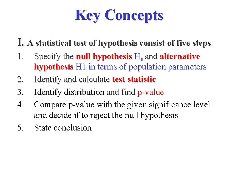
Key Concepts I. A statistical test of hypothesis consist of five steps 1. 2. 3. 4. 5. Specify the null hypothesis H 0 and alternative hypothesis H 1 in terms of population parameters Identify and calculate test statistic Identify distribution and find p-value Compare p-value with the given significance level and decide if to reject the null hypothesis State conclusion

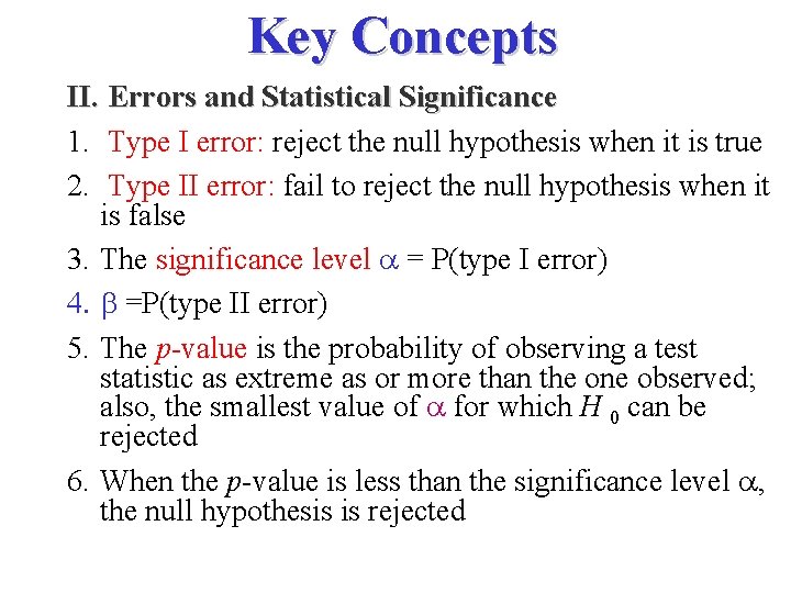
Key Concepts II. Errors and Statistical Significance 1. Type I error: reject the null hypothesis when it is true 2. Type II error: fail to reject the null hypothesis when it is false 3. The significance level = P(type I error) 4. =P(type II error) 5. The p-value is the probability of observing a test statistic as extreme as or more than the one observed; also, the smallest value of for which H 0 can be rejected 6. When the p-value is less than the significance level , the null hypothesis is rejected

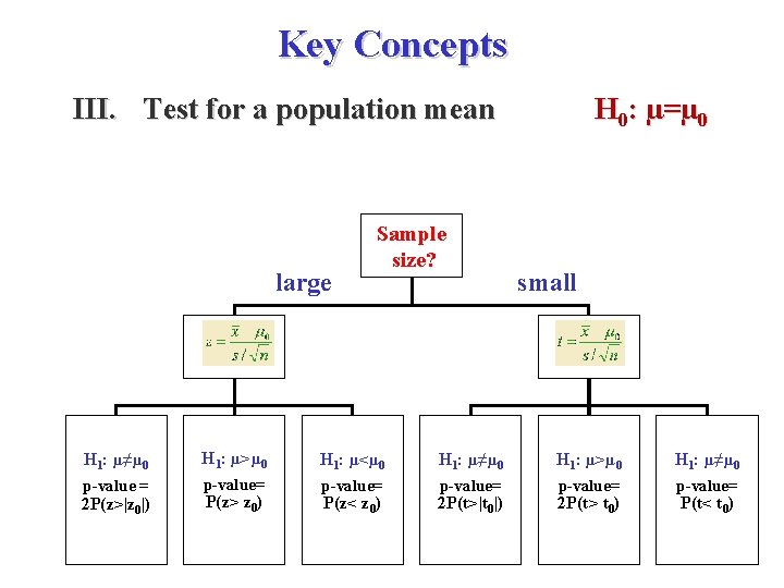
Key Concepts III. Test for a population mean H 0: µ=µ 0 Sample size? large small H 1: µ≠µ 0 H 1: µ>µ 0 H 1: µ<µ 0 H 1: µ≠µ 0 H 1: µ>µ 0 H 1: µ≠µ 0 p-value = p-value= p-value= 2 P(z>|z 0|) P(z> z 0) P(z< z 0) 2 P(t>|t 0|) 2 P(t> t 0) P(t< t 0)

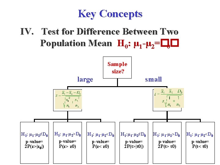
Key Concepts IV. Test for Difference Between Two Population Mean H 0: µ 1 -µ 2=�� 0 Sample size? large small H 1: µ 1 -µ 2≠D 0 H 1: µ 1 -µ 2>D 0 H 1: µ 1 -µ 2<D 0 H 1: µ 1 -µ 2≠D 0 H 1: µ 1 -µ 2>D 0 H 1: µ 1 -µ 2<D 0 p-value= p-value= 2 P(z>|z 0|) P(z> z 0) P(z< z 0) 2 P(t>|t 0|) 2 P(t> t 0) P(t< t 0)

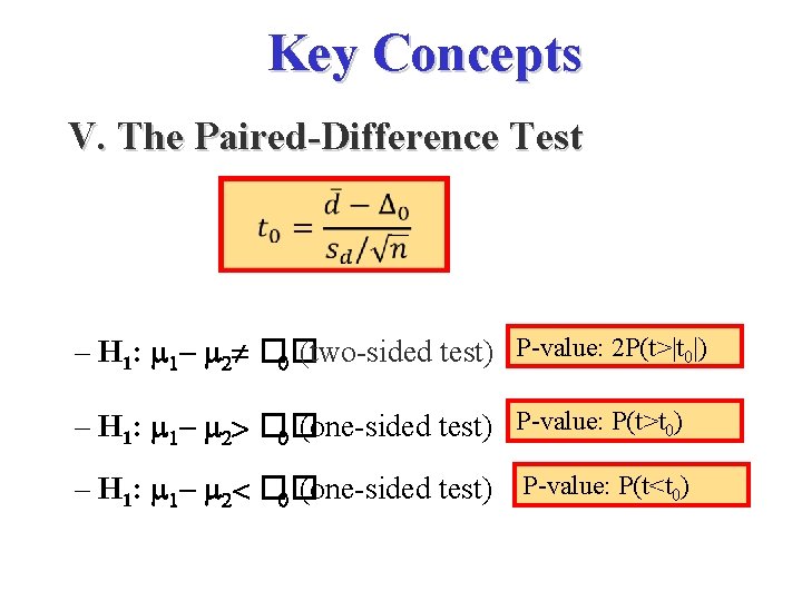
Key Concepts V. The Paired-Difference Test P-value: 2 P(t>|t 0|) – H 1: m 1 - m 2 �� (two-sided test) 0 P-value: P(t>t 0) – H 1: m 1 - m 2> �� 0 (one-sided test) P-value: P(t<t 0) – H 1: m 1 - m 2< �� 0 (one-sided test)