AP Statistics Exam Review CHAPTERS 6 8 Chapter

AP Statistics Exam Review CHAPTERS 6 -8

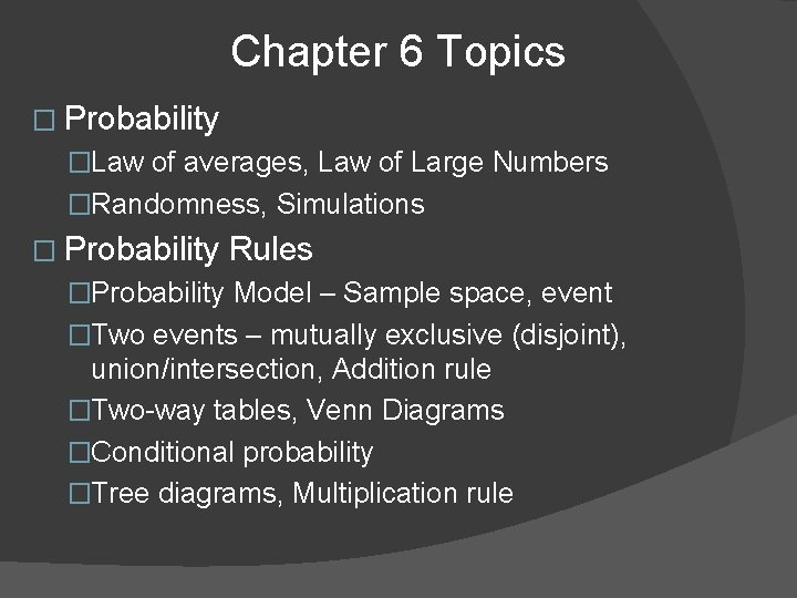
Chapter 6 Topics � Probability �Law of averages, Law of Large Numbers �Randomness, Simulations � Probability Rules �Probability Model – Sample space, event �Two events – mutually exclusive (disjoint), union/intersection, Addition rule �Two-way tables, Venn Diagrams �Conditional probability �Tree diagrams, Multiplication rule

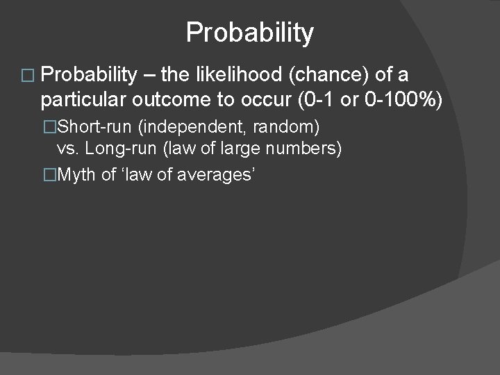
Probability � Probability – the likelihood (chance) of a particular outcome to occur (0 -1 or 0 -100%) �Short-run (independent, random) vs. Long-run (law of large numbers) �Myth of ‘law of averages’

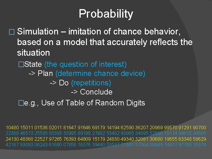
Probability � Simulation – imitation of chance behavior, based on a model that accurately reflects the situation �State (the question of interest) -> Plan (determine chance device) -> Do (repetitions) -> Conclude �e. g. , Use of Table of Random Digits 10480 15011 01536 02011 81647 91646 69179 14194 62590 36207 20969 99570 91291 90700 22368 46573 25595 85393 30995 89198 27982 53402 93965 34095 52666 19174 39615 99505 24130 48360 22527 97265 76393 64809 15179 24830 49340 32081 30680 19655 63348 58629 42167 93093 06243 61680 07856 16376 39440 53537 71341 57004 00849 74917 97758 16379

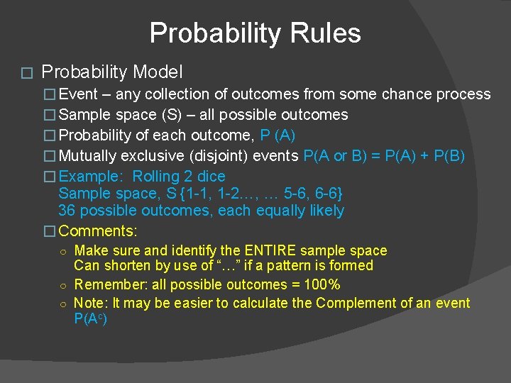
Probability Rules � Probability Model � Event – any collection of outcomes from some chance process � Sample space (S) – all possible outcomes � Probability of each outcome, P (A) � Mutually exclusive (disjoint) events P(A or B) = P(A) + P(B) � Example: Rolling 2 dice Sample space, S {1 -1, 1 -2…, … 5 -6, 6 -6} 36 possible outcomes, each equally likely � Comments: ○ Make sure and identify the ENTIRE sample space Can shorten by use of “…” if a pattern is formed ○ Remember: all possible outcomes = 100% ○ Note: It may be easier to calculate the Complement of an event P(Ac)

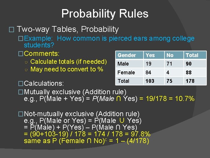
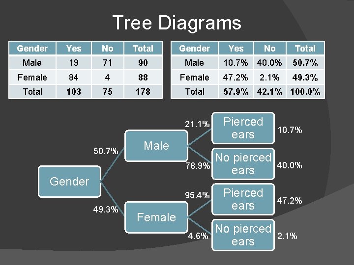
Probability Rules � Two-way Tables, Probability �Example: How common is pierced ears among college students? �Comments: ○ Calculate totals (if needed) ○ May need to convert to % Gender Yes No Total Male 19 71 90 Female 84 4 88 103 75 178 Total �Calculations: �Mutually exclusive (Addition rule) e. g. , P(Male + Yes) = P(Male ∩ Yes) = 19/178 = 10. 7% �Not-mutually exclusive (Addition rule) e. g. , P(Male or Yes) = P(Male ∪ Yes) = P(Male) + P(Yes) – P(Male ∩ Yes) = (90+103 -19) / 178 = 174 / 178 = 97. 8% same as P (Female ∩ No)c = 1 – (4/178)

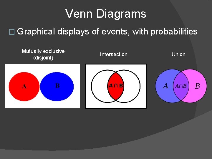
Venn Diagrams � Graphical displays of events, with probabilities Mutually exclusive (disjoint) Intersection A∩B Union

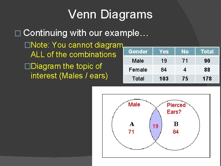
Venn Diagrams � Continuing with our example… �Note: You cannot diagram ALL of the combinations �Diagram the topic of interest (Males / ears) Gender Yes No Total Male 19 71 90 Female 84 4 88 Total 103 75 178 Male 71 Pierced Ears? 19 84

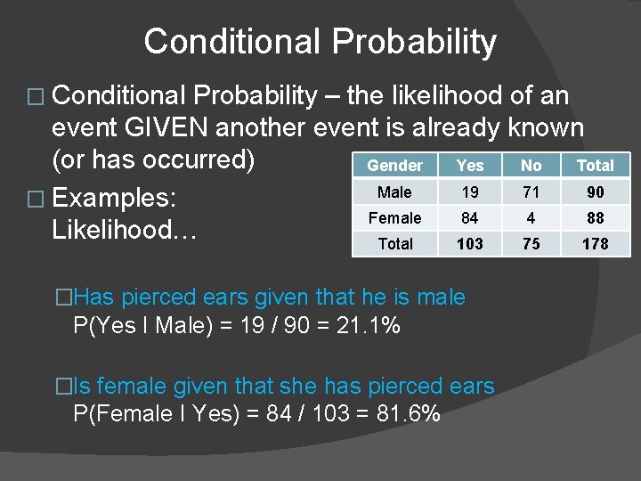
Conditional Probability � Conditional Probability – the likelihood of an event GIVEN another event is already known (or has occurred) Gender Yes No Total Male 19 71 90 � Examples: Female 84 4 88 Likelihood… Total 103 75 178 �Has pierced ears given that he is male P(Yes I Male) = 19 / 90 = 21. 1% �Is female given that she has pierced ears P(Female I Yes) = 84 / 103 = 81. 6%

Tree Diagrams Gender Yes No Total Gender Male 19 71 90 Male Female 84 4 88 Female Total 103 75 178 Total 57. 9% 42. 1% 100. 0% 21. 1% Pierced ears 10. 7% 78. 9% No pierced ears 40. 0% 95. 4% Pierced ears 47. 2% 4. 6% No pierced ears 2. 1% 50. 7% Male Gender 49. 3% Female Yes No Total 10. 7% 40. 0% 50. 7% 47. 2% 49. 3% 2. 1%

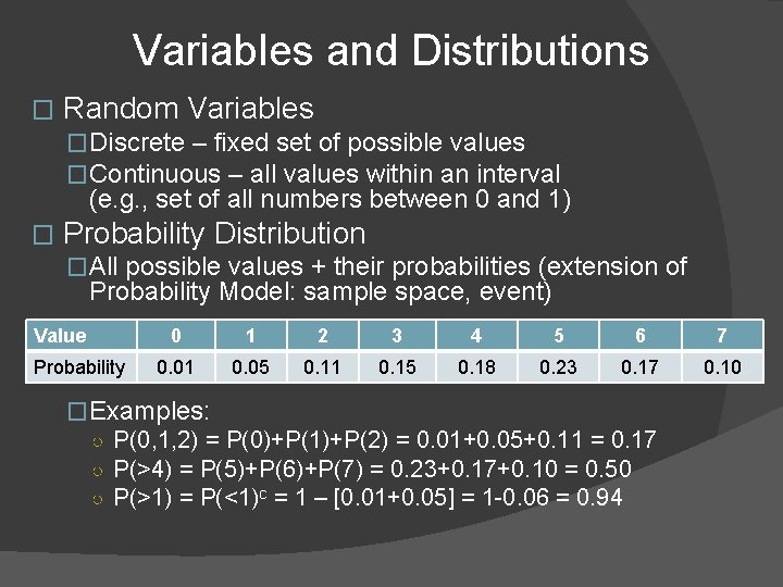
Variables and Distributions � Random Variables �Discrete – fixed set of possible values �Continuous – all values within an interval (e. g. , set of all numbers between 0 and 1) � Probability Distribution �All possible values + their probabilities (extension of Probability Model: sample space, event) Value � Probability 0 1 2 3 4 5 6 7 0. 01 0. 05 0. 11 0. 15 0. 18 0. 23 0. 17 0. 10 �Examples: ○ P(0, 1, 2) = P(0)+P(1)+P(2) = 0. 01+0. 05+0. 11 = 0. 17 ○ P(>4) = P(5)+P(6)+P(7) = 0. 23+0. 17+0. 10 = 0. 50 ○ P(>1) = P(<1)c = 1 – [0. 01+0. 05] = 1 -0. 06 = 0. 94

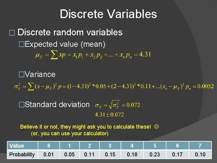
Discrete Variables � Discrete random variables �Expected value (mean) �Variance �Standard deviation Believe it or not, they might ask you to calculate these! (or, you can use your calculator) Value Probability 0 1 2 3 4 5 6 7 0. 01 0. 05 0. 11 0. 15 0. 18 0. 23 0. 17 0. 10

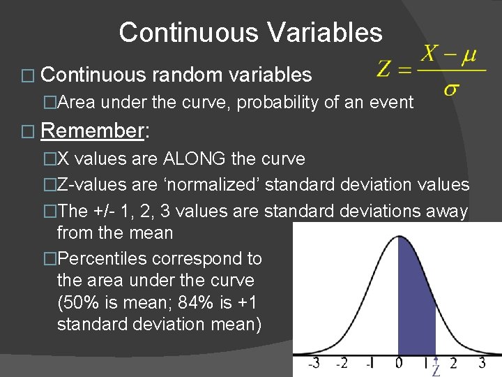
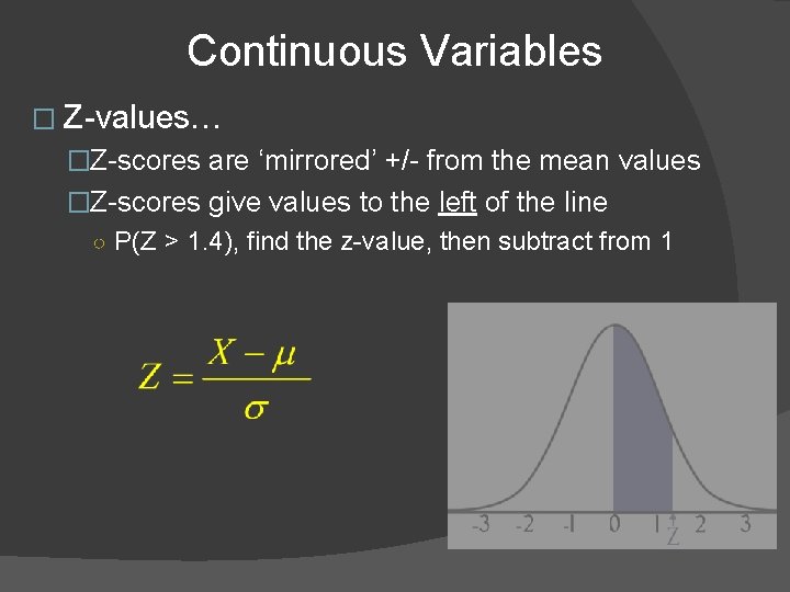
Continuous Variables � Continuous random variables �Area under the curve, probability of an event � Remember: �X values are ALONG the curve �Z-values are ‘normalized’ standard deviation values �The +/- 1, 2, 3 values are standard deviations away from the mean �Percentiles correspond to the area under the curve (50% is mean; 84% is +1 standard deviation mean)

Continuous Variables � Z-values… �Z-scores are ‘mirrored’ +/- from the mean values �Z-scores give values to the left of the line ○ P(Z > 1. 4), find the z-value, then subtract from 1

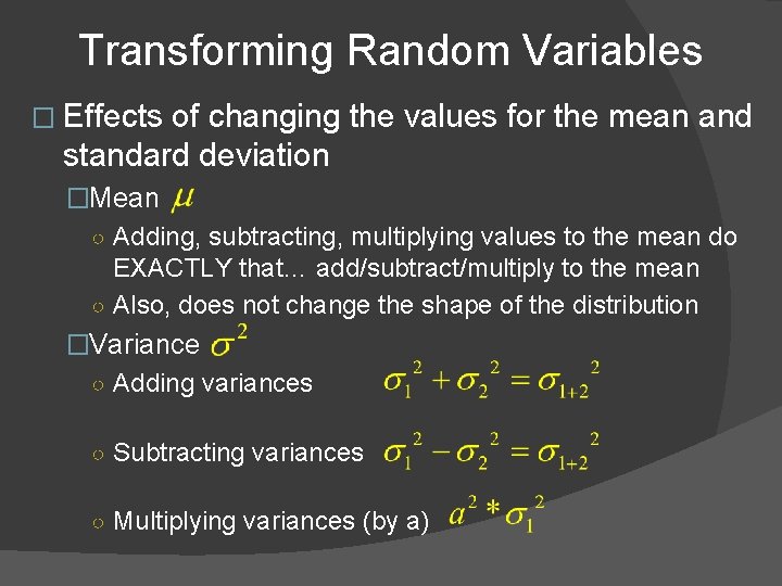
Transforming Random Variables � Effects of changing the values for the mean and standard deviation �Mean ○ Adding, subtracting, multiplying values to the mean do EXACTLY that… add/subtract/multiply to the mean ○ Also, does not change the shape of the distribution �Variance ○ Adding variances ○ Subtracting variances ○ Multiplying variances (by a)

Transforming Random Variables � Effects of changing the values for the mean and standard deviation �Standard deviation ○ For adding, subtracting, multiplying standard deviations �They operate in the same manner as variances but… �You MUST work with variances 1 st… then take the square-root of the values! �Also, changing the variance (and standard deviation) values by adding/subtracting/multiplying DOES change the shape

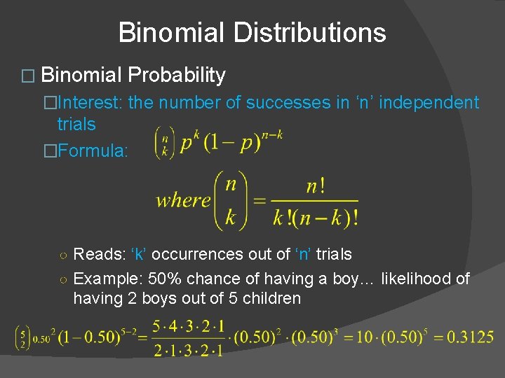
Binomial Distributions � Binomial �Perform several independent trials of the same chance process and record number of times a particular outcome occurs �Examples: ○ Toss a coin 5 times ○ Spin a roulette wheel 10 times ○ Random sample of 100 babies born in U. S. �Sample problems: ○ Shuffle deck, turn over top card, repeat 10 times, count how many aces are observed ○ Choose students at random and identify how many are taller than 6 feet ○ Flip a coin, repeat 20 times, count how many heads are observed

Binomial Distributions � Binomial Probability �Interest: the number of successes in ‘n’ independent trials �Formula: ○ Reads: ‘k’ occurrences out of ‘n’ trials ○ Example: 50% chance of having a boy… likelihood of having 2 boys out of 5 children

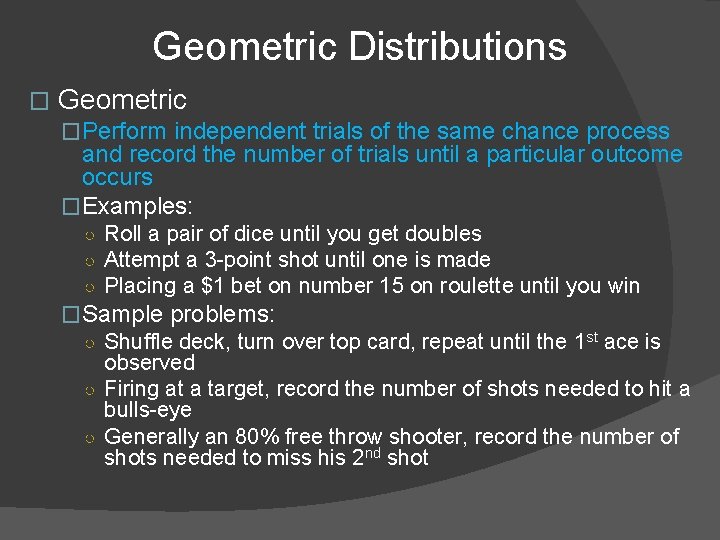
Geometric Distributions � Geometric �Perform independent trials of the same chance process and record the number of trials until a particular outcome occurs �Examples: ○ Roll a pair of dice until you get doubles ○ Attempt a 3 -point shot until one is made ○ Placing a $1 bet on number 15 on roulette until you win �Sample problems: ○ Shuffle deck, turn over top card, repeat until the 1 st ace is observed ○ Firing at a target, record the number of shots needed to hit a bulls-eye ○ Generally an 80% free throw shooter, record the number of shots needed to miss his 2 nd shot

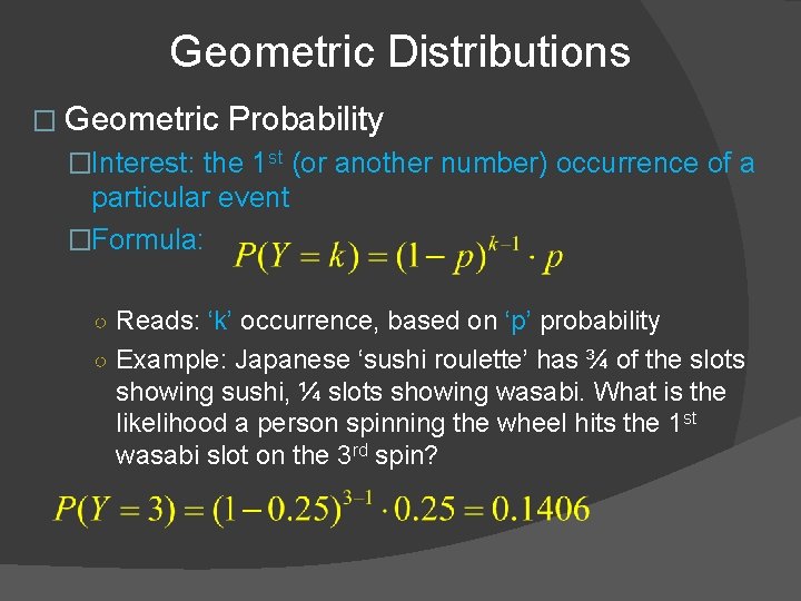
Geometric Distributions � Geometric Probability �Interest: the 1 st (or another number) occurrence of a particular event �Formula: ○ Reads: ‘k’ occurrence, based on ‘p’ probability ○ Example: Japanese ‘sushi roulette’ has ¾ of the slots showing sushi, ¼ slots showing wasabi. What is the likelihood a person spinning the wheel hits the 1 st wasabi slot on the 3 rd spin?

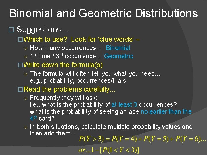
Binomial and Geometric Distributions � Suggestions… �Which to use? Look for ‘clue words’ – ○ How many occurrences… Binomial ○ 1 st time / 3 rd occurrence… Geometric �Write down the formula(s) ○ The formula will often tell you what you need… e. g. , probability, occurrences/trials �Read the problems carefully… ○ Frequently they will ask: i. e. , what is the probability of at least 3 occurrences? what is the probability of seeing an ace no earlier than the 4 th card? ○ In both situations, calculate multiple probability values and then add them…