ENGR 201 Statistics for Engineers Chapter 4 Continuous

ENGR 201: Statistics for Engineers Chapter 4 Continuous Random Variables and Probability Distributions* Normal and Other Continuous Probability Distributions *Partly based on the lecture notes of Y. Wang of UCLA and of D. Tenenbaum of UNC Note 7 of 5 E

Review I. What’s in last lecture? Binomial, Poisson and Hypergeometric Probability Distributions. Chapter 3. II. What's in this lecture? Normal and Other Continuous Probability Distributions. Read Chapter 4 Note 7 of 5 E

Continuous Random Variables • A random variable is continuous if it can assume the infinitely many values corresponding to points on a line interval, e. g. , heights, weights, p. H, velocity, temperature. • Some random variables that are technically discrete exhibit such a tremendous range of values, that it is desirable to treat them as if they were continuous variables, e. g. , population • Continuous random variables are described by probability density functions (PDFs) Note 7 of 5 E

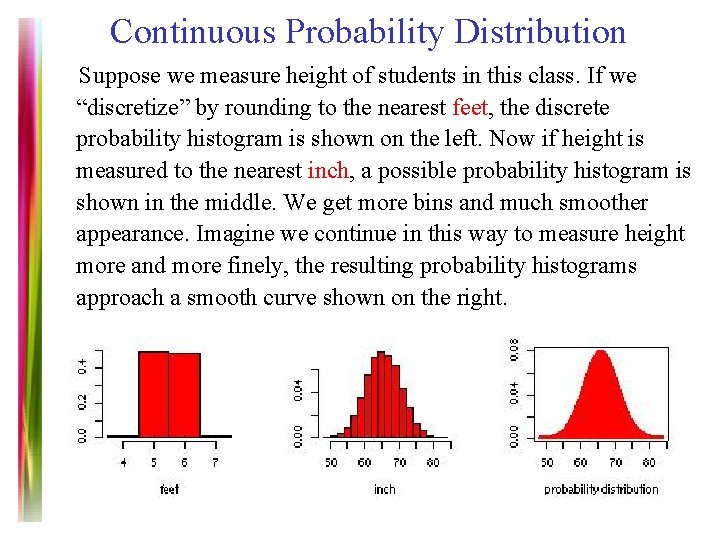
Continuous Probability Distribution Suppose we measure height of students in this class. If we “discretize” by rounding to the nearest feet, the discrete probability histogram is shown on the left. Now if height is measured to the nearest inch, a possible probability histogram is shown in the middle. We get more bins and much smoother appearance. Imagine we continue in this way to measure height more and more finely, the resulting probability histograms approach a smooth curve shown on the right. Note 7 of 5 E

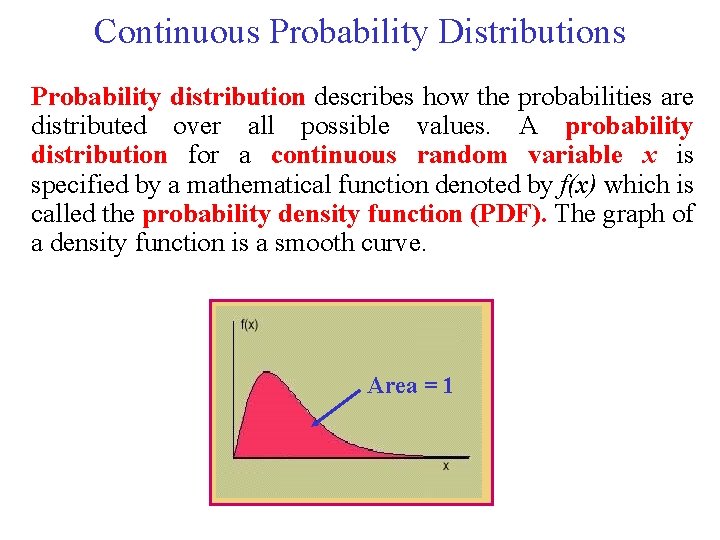
Continuous Probability Distributions Probability distribution describes how the probabilities are distributed over all possible values. A probability distribution for a continuous random variable x is specified by a mathematical function denoted by f(x) which is called the probability density function (PDF). The graph of a density function is a smooth curve. Area = 1 Note 7 of 5 E

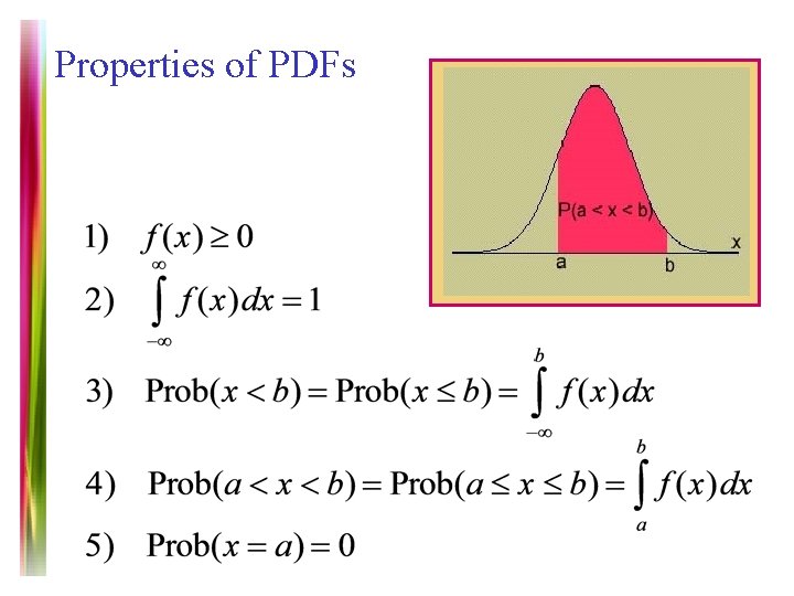
Properties of PDFs Note 7 of 5 E

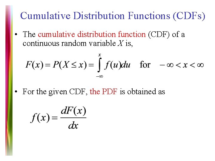
Cumulative Distribution Functions (CDFs) • The cumulative distribution function (CDF) of a continuous random variable X is, • For the given CDF, the PDF is obtained as Note 7 of 5 E

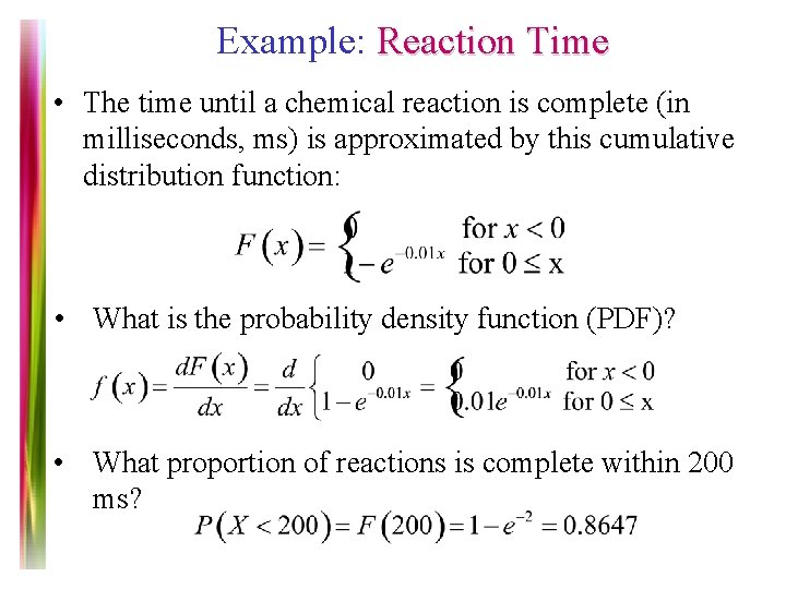
Example: Reaction Time • The time until a chemical reaction is complete (in milliseconds, ms) is approximated by this cumulative distribution function: • What is the probability density function (PDF)? • What proportion of reactions is complete within 200 ms? Note 7 of 5 E

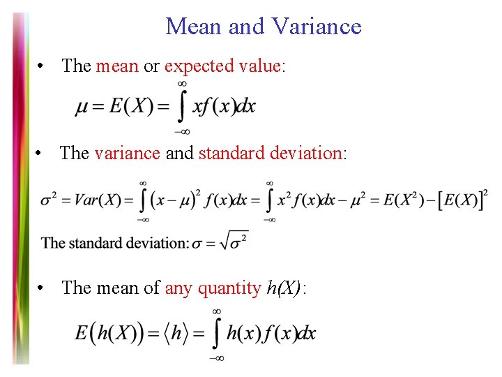
Mean and Variance • The mean or expected value: • The variance and standard deviation: • The mean of any quantity h(X): Note 7 of 5 E

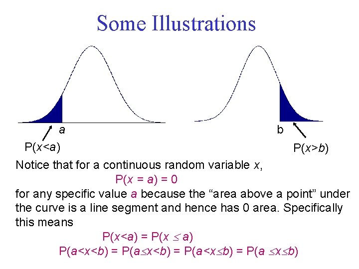
Some Illustrations a P(x<a) b P(x>b) Notice that for a continuous random variable x, P(x = a) = 0 for any specific value a because the “area above a point” under the curve is a line segment and hence has 0 area. Specifically this means P(x<a) = P(x a) P(a<x<b) = P(a<x b) = P(a x b)Note 7 of 5 E

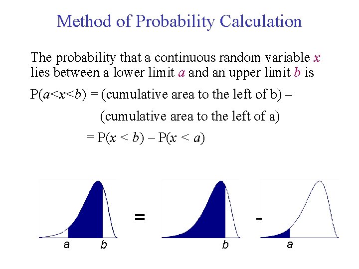
Method of Probability Calculation The probability that a continuous random variable x lies between a lower limit a and an upper limit b is P(a<x<b) = (cumulative area to the left of b) – (cumulative area to the left of a) = P(x < b) – P(x < a) = a b b a Note 7 of 5 E

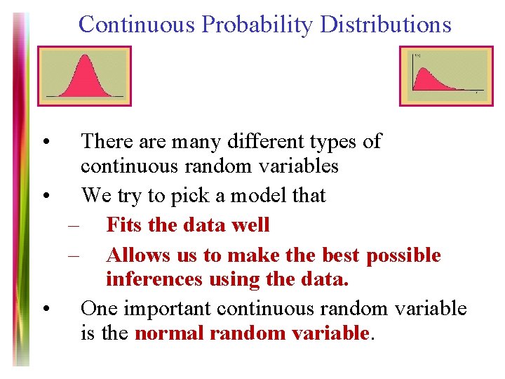
Continuous Probability Distributions • There are many different types of continuous random variables • We try to pick a model that – Fits the data well – Allows us to make the best possible inferences using the data. • One important continuous random variable is the normal random variable. Note 7 of 5 E

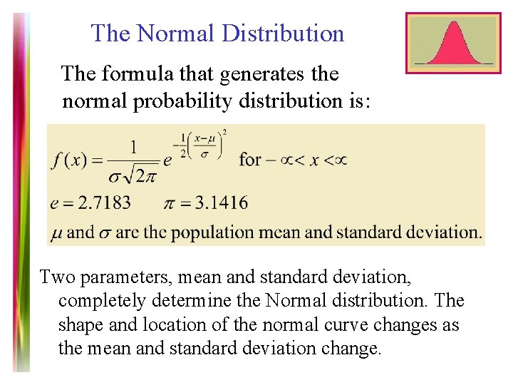
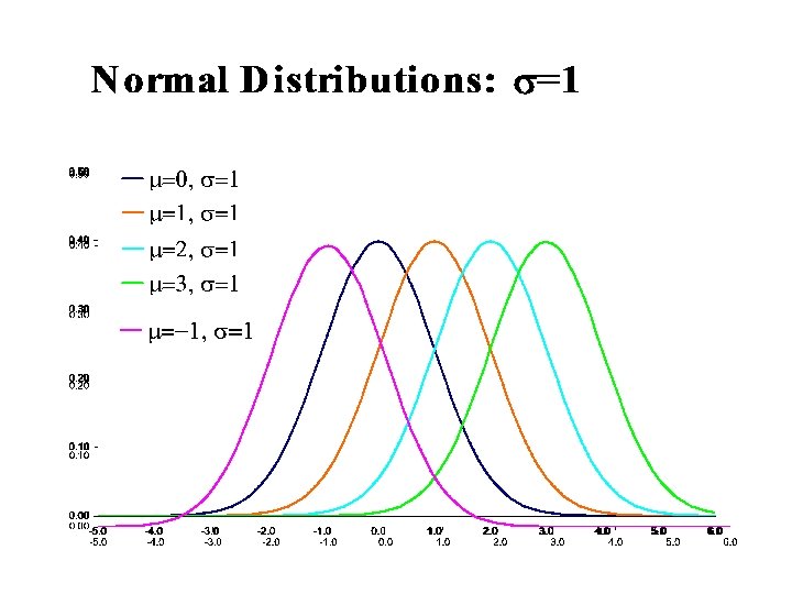
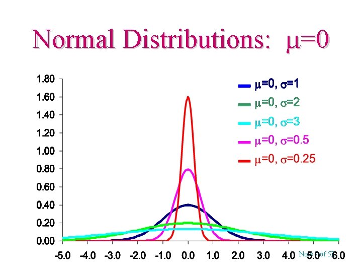
The Normal Distribution The formula that generates the normal probability distribution is: Two parameters, mean and standard deviation, completely determine the Normal distribution. The shape and location of the normal curve changes as the mean and standard deviation change. Note 7 of 5 E

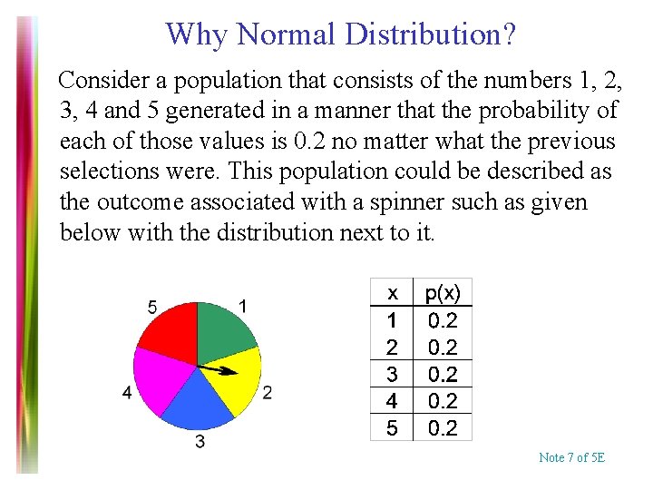
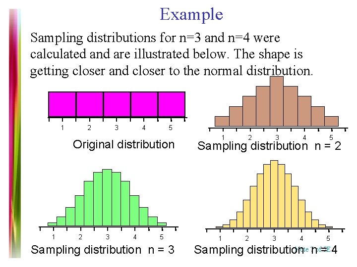
Why Normal Distribution? Consider a population that consists of the numbers 1, 2, 3, 4 and 5 generated in a manner that the probability of each of those values is 0. 2 no matter what the previous selections were. This population could be described as the outcome associated with a spinner such as given below with the distribution next to it. Note 7 of 5 E

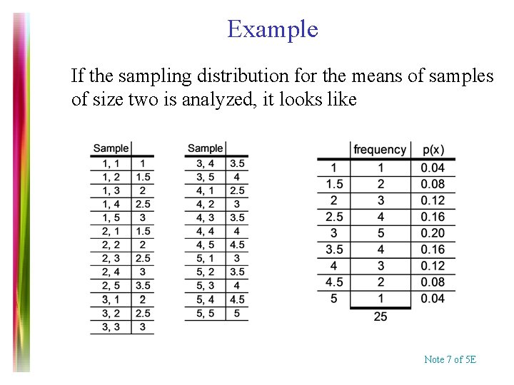
Example If the sampling distribution for the means of samples of size two is analyzed, it looks like Note 7 of 5 E

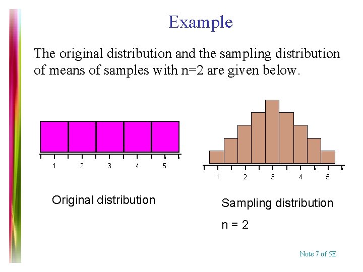
Example The original distribution and the sampling distribution of means of samples with n=2 are given below. 1 2 3 4 5 1 Original distribution 2 3 4 5 Sampling distribution n=2 Note 7 of 5 E

Example Sampling distributions for n=3 and n=4 were calculated and are illustrated below. The shape is getting closer and closer to the normal distribution. 1 2 3 4 5 Original distribution 1 2 3 4 5 Sampling distribution n = 3 1 2 3 4 5 Sampling distribution n = 2 1 2 3 4 5 Note 7 nof= 5 E 4 Sampling distribution

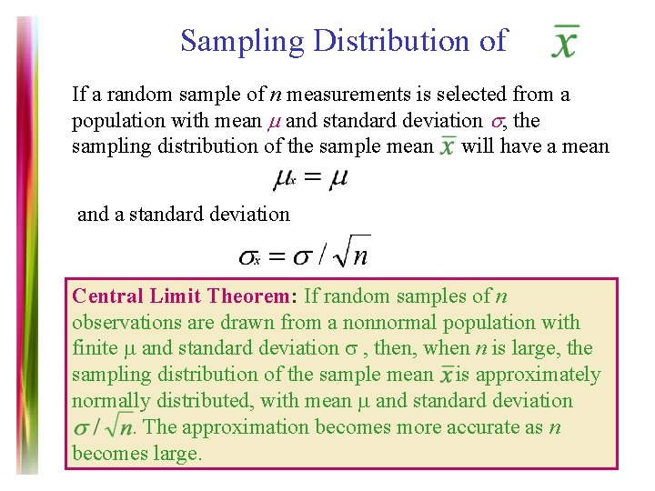
Sampling Distribution of If a random sample of n measurements is selected from a population with mean m and standard deviation s, the sampling distribution of the sample mean will have a mean and a standard deviation Central Limit Theorem: If random samples of n observations are drawn from a nonnormal population with finite and standard deviation , then, when n is large, the sampling distribution of the sample mean is approximately normally distributed, with mean and standard deviation. The approximation becomes more accurate as n becomes large. Note 7 of 5 E

Note 7 of 5 E

Normal Distributions: =0 Note 7 of 5 E

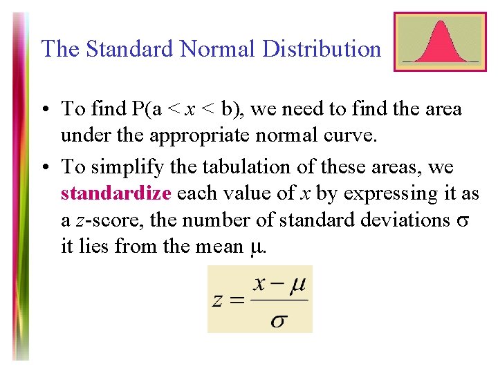
The Standard Normal Distribution • To find P(a < x < b), we need to find the area under the appropriate normal curve. • To simplify the tabulation of these areas, we standardize each value of x by expressing it as a z-score, the number of standard deviations it lies from the mean . Note 7 of 5 E

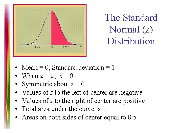
The Standard Normal (z) Distribution • • Mean = 0; Standard deviation = 1 When x = , z = 0 Symmetric about z = 0 Values of z to the left of center are negative Values of z to the right of center are positive Total area under the curve is 1. Areas on both sides of center equal to 0. 5 Note 7 of 5 E

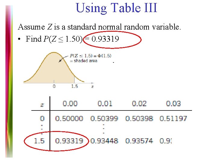
Using Table III Assume Z is a standard normal random variable. • Find P(Z ≤ 1. 50) = 0. 93319 Note 7 of 5 E

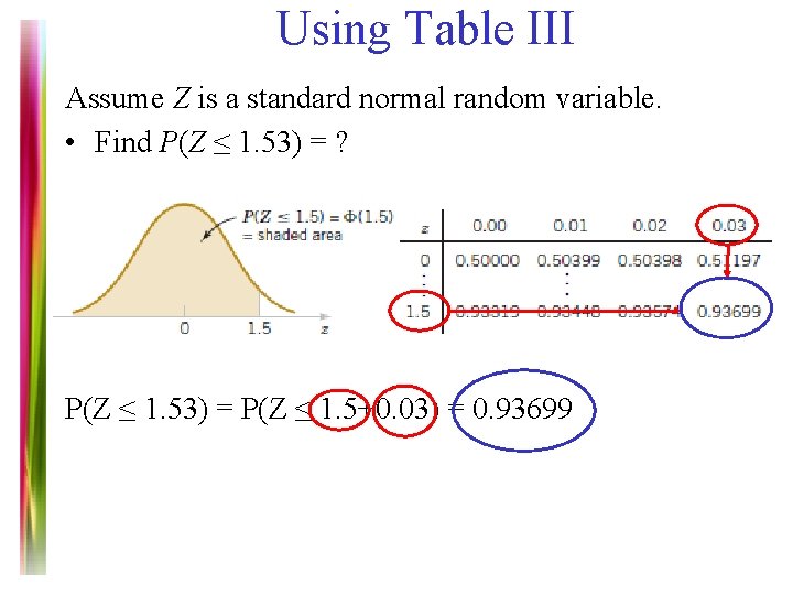
Using Table III Assume Z is a standard normal random variable. • Find P(Z ≤ 1. 53) = ? P(Z ≤ 1. 53) = P(Z ≤ 1. 5+0. 03) = 0. 93699 Note 7 of 5 E

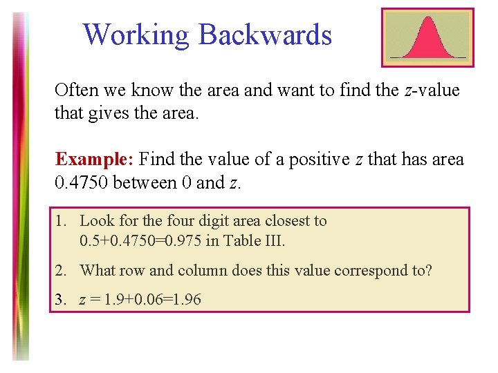
Working Backwards Often we know the area and want to find the z-value that gives the area. Example: Find the value of a positive z that has area 0. 4750 between 0 and z. 1. Look for the four digit area closest to 0. 5+0. 4750=0. 975 in Table III. 2. What row and column does this value correspond to? 3. z = 1. 9+0. 06=1. 96 Note 7 of 5 E

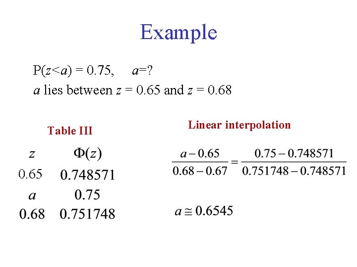
Example P(z<a) = 0. 75, a=? a lies between z = 0. 65 and z = 0. 68 Table III Linear interpolation 0. 65 Note 7 of 5 E

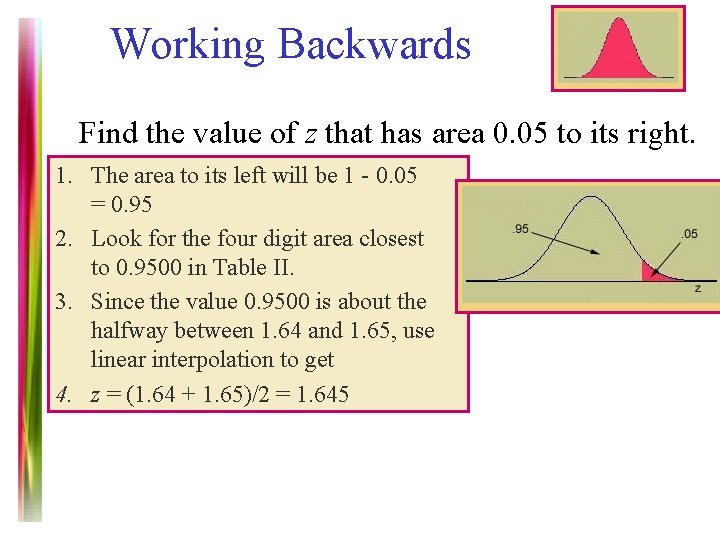
Working Backwards Find the value of z that has area 0. 05 to its right. 1. The area to its left will be 1 - 0. 05 = 0. 95 2. Look for the four digit area closest to 0. 9500 in Table II. 3. Since the value 0. 9500 is about the halfway between 1. 64 and 1. 65, use linear interpolation to get 4. z = (1. 64 + 1. 65)/2 = 1. 645 Note 7 of 5 E

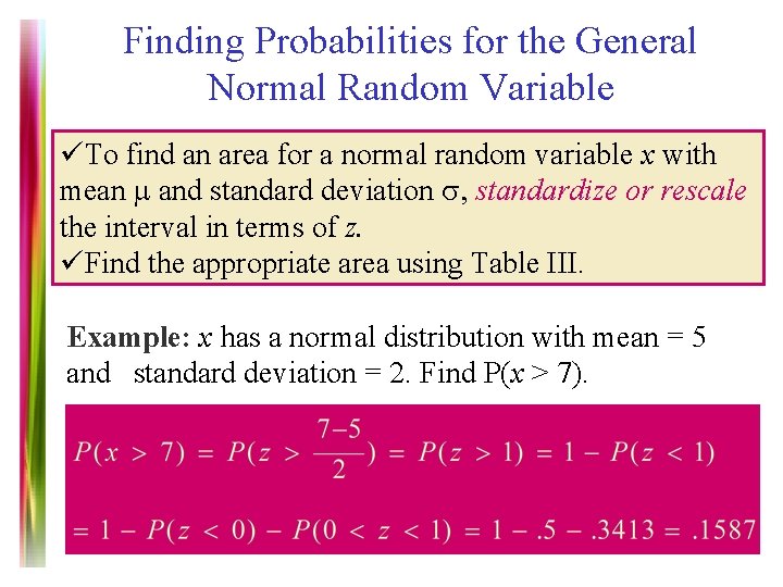
Finding Probabilities for the General Normal Random Variable üTo find an area for a normal random variable x with mean and standard deviation , standardize or rescale the interval in terms of z. üFind the appropriate area using Table III. Example: x has a normal distribution with mean = 5 and standard deviation = 2. Find P(x > 7). Note 7 of 5 E

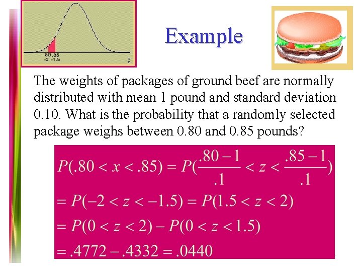
Example The weights of packages of ground beef are normally distributed with mean 1 pound and standard deviation 0. 10. What is the probability that a randomly selected package weighs between 0. 80 and 0. 85 pounds? Note 7 of 5 E

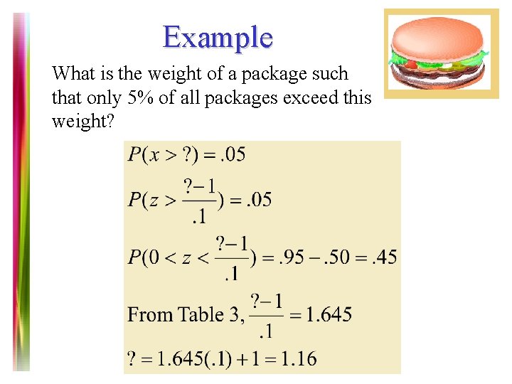
Example What is the weight of a package such that only 5% of all packages exceed this weight? Note 7 of 5 E

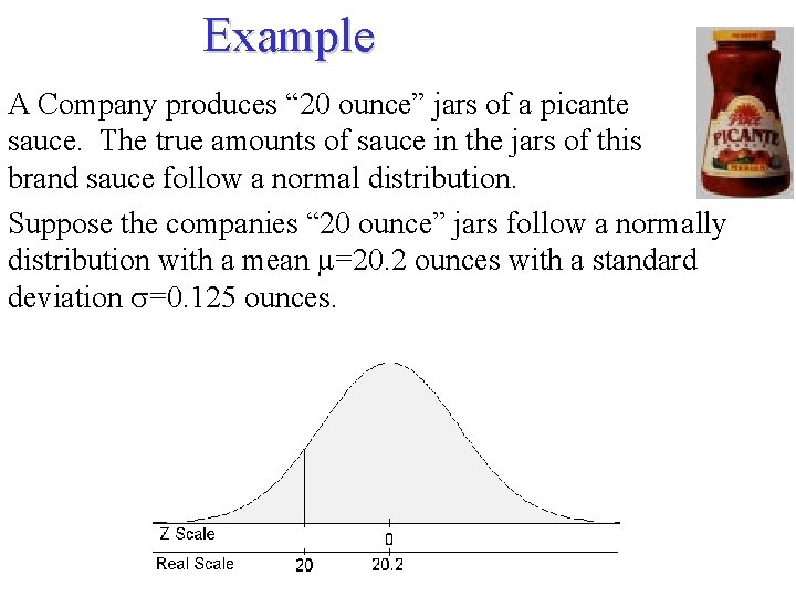
Example A Company produces “ 20 ounce” jars of a picante sauce. The true amounts of sauce in the jars of this brand sauce follow a normal distribution. Suppose the companies “ 20 ounce” jars follow a normally distribution with a mean =20. 2 ounces with a standard deviation =0. 125 ounces. Note 7 of 5 E

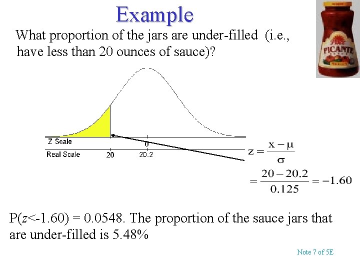
Example What proportion of the jars are under-filled (i. e. , have less than 20 ounces of sauce)? P(z<-1. 60) = 0. 0548. The proportion of the sauce jars that are under-filled is 5. 48% Note 7 of 5 E

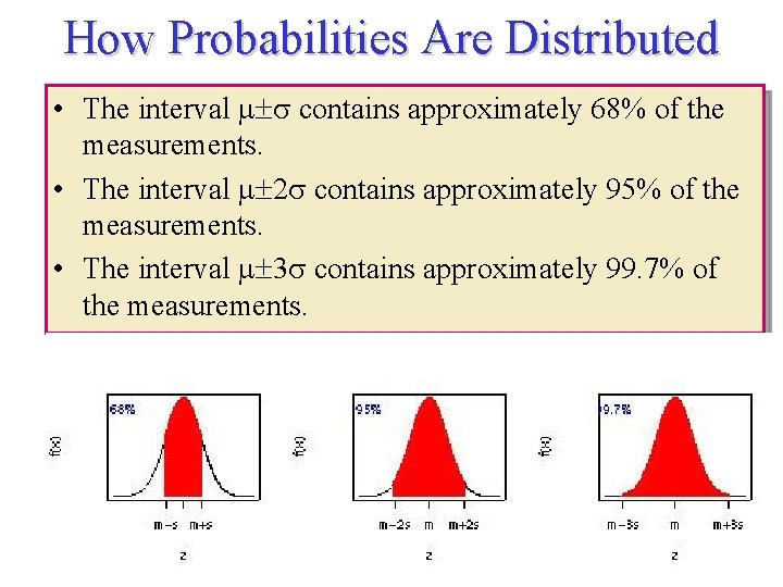
How Probabilities Are Distributed • The interval contains approximately 68% of the measurements. • The interval 2 contains approximately 95% of the measurements. • The interval 3 contains approximately 99. 7% of the measurements. Note 7 of 5 E

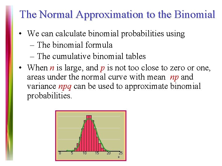
The Normal Approximation to the Binomial • We can calculate binomial probabilities using – The binomial formula – The cumulative binomial tables • When n is large, and p is not too close to zero or one, areas under the normal curve with mean np and variance npq can be used to approximate binomial probabilities. Note 7 of 5 E

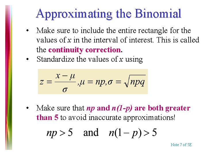
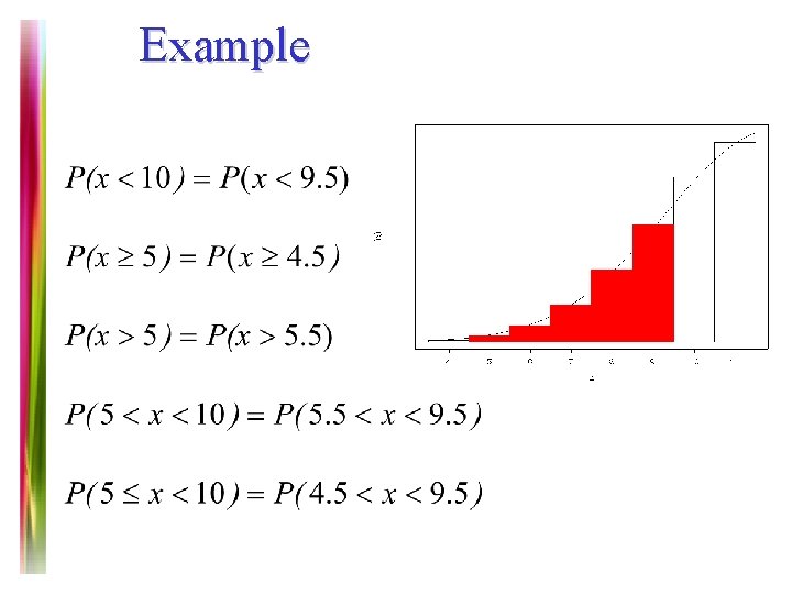
Approximating the Binomial • Make sure to include the entire rectangle for the values of x in the interval of interest. This is called the continuity correction. • Standardize the values of x using • Make sure that np and n(1 -p) are both greater than 5 to avoid inaccurate approximations! Note 7 of 5 E

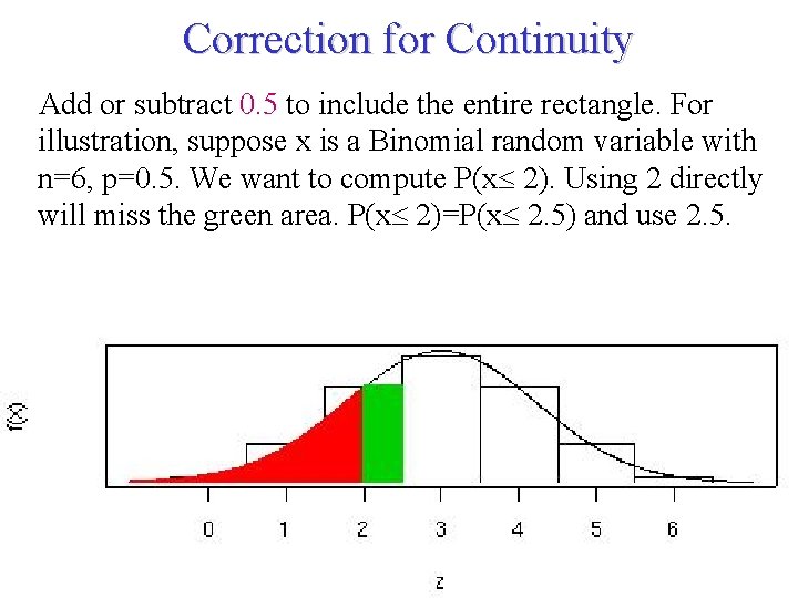
Correction for Continuity Add or subtract 0. 5 to include the entire rectangle. For illustration, suppose x is a Binomial random variable with n=6, p=0. 5. We want to compute P(x 2). Using 2 directly will miss the green area. P(x 2)=P(x 2. 5) and use 2. 5. Note 7 of 5 E

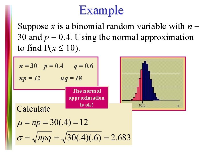
Example Suppose x is a binomial random variable with n = 30 and p = 0. 4. Using the normal approximation to find P(x 10). n = 30 np = 12 p = 0. 4 q = 0. 6 nq = 18 The normal approximation is ok! Note 7 of 5 E

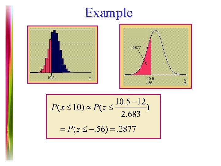
Example Note 7 of 5 E

Example Note 7 of 5 E

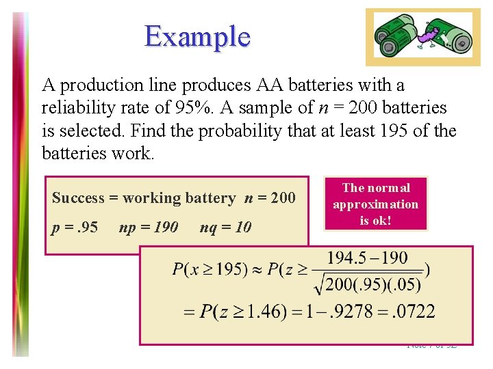
Example A production line produces AA batteries with a reliability rate of 95%. A sample of n = 200 batteries is selected. Find the probability that at least 195 of the batteries work. Success = working battery n = 200 p =. 95 np = 190 nq = 10 The normal approximation is ok! Note 7 of 5 E

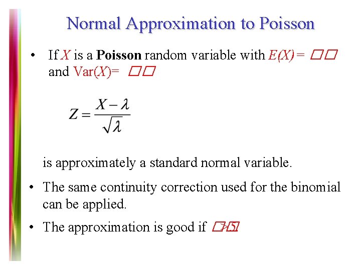
Normal Approximation to Poisson • If X is a Poisson random variable with E(X)= �� and Var(X)= �� is approximately a standard normal variable. • The same continuity correction used for the binomial can be applied. • The approximation is good if �� >5. Note 7 of 5 E

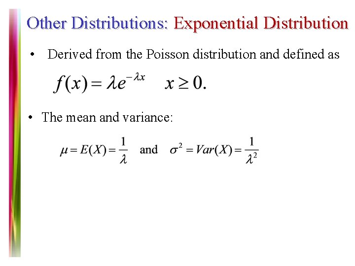
Other Distributions: Exponential Distribution • Derived from the Poisson distribution and defined as • The mean and variance: Note 7 of 5 E

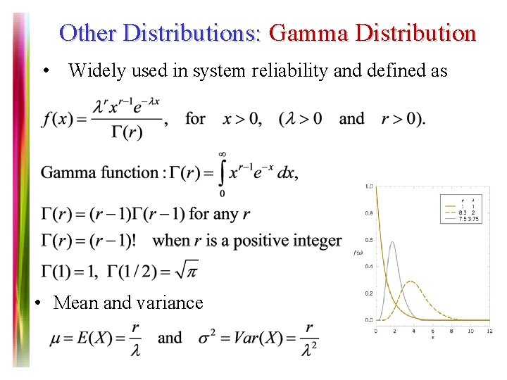
Other Distributions: Gamma Distribution • Widely used in system reliability and defined as • Mean and variance Note 7 of 5 E

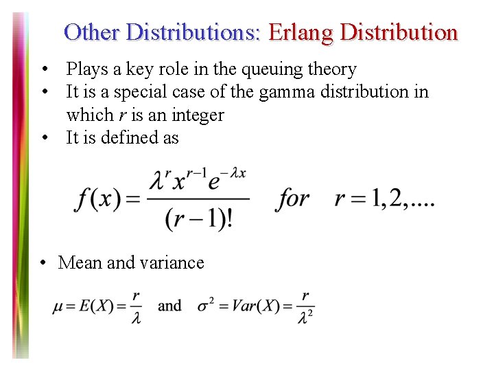
Other Distributions: Erlang Distribution • Plays a key role in the queuing theory • It is a special case of the gamma distribution in which r is an integer • It is defined as • Mean and variance Note 7 of 5 E

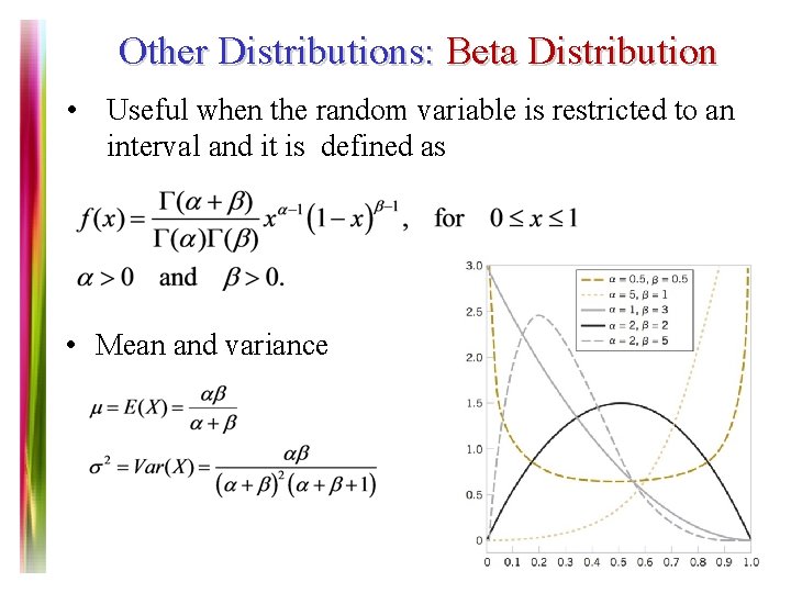
Other Distributions: Beta Distribution • Useful when the random variable is restricted to an interval and it is defined as • Mean and variance Note 7 of 5 E

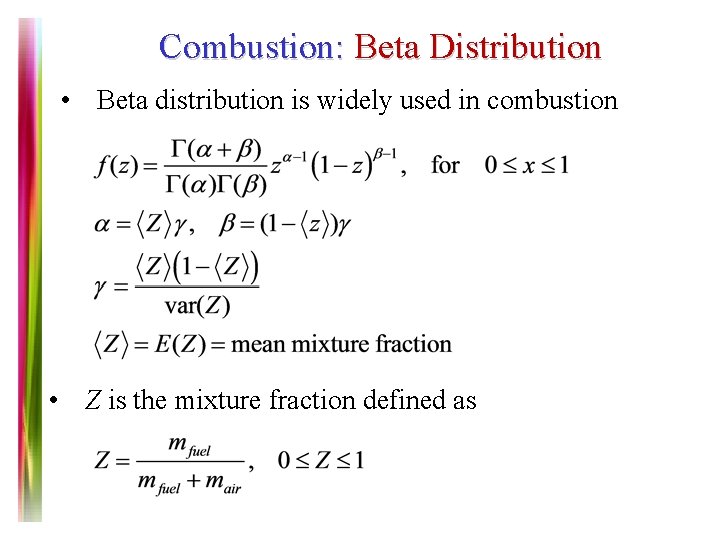
Combustion: Beta Distribution • Beta distribution is widely used in combustion • Z is the mixture fraction defined as Note 7 of 5 E

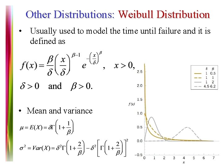
Other Distributions: Weibull Distribution • Usually used to model the time until failure and it is defined as • Mean and variance Note 7 of 5 E

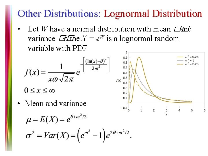
Other Distributions: Lognormal Distribution • Let W have a normal distribution with mean �� and 2; the X = e. W is a lognormal random variance �� variable with PDF • Mean and variance Note 7 of 5 E

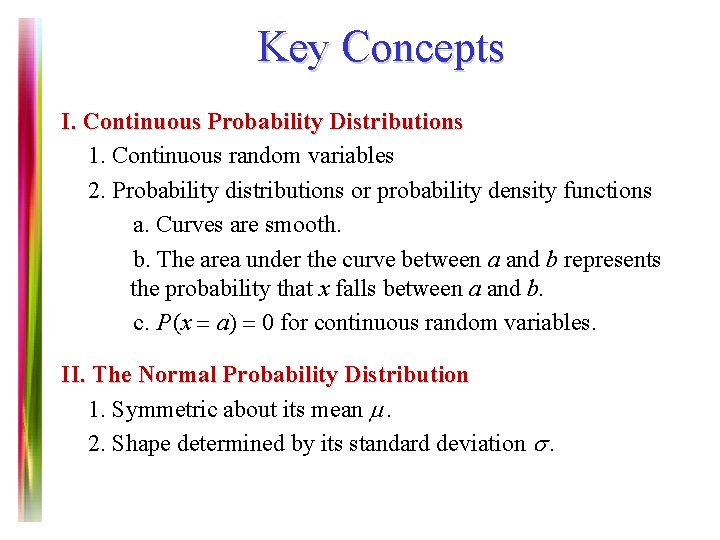
Key Concepts I. Continuous Probability Distributions 1. Continuous random variables 2. Probability distributions or probability density functions a. Curves are smooth. b. The area under the curve between a and b represents the probability that x falls between a and b. c. P (x = a) = 0 for continuous random variables. II. The Normal Probability Distribution 1. Symmetric about its mean m. 2. Shape determined by its standard deviation s. Note 7 of 5 E

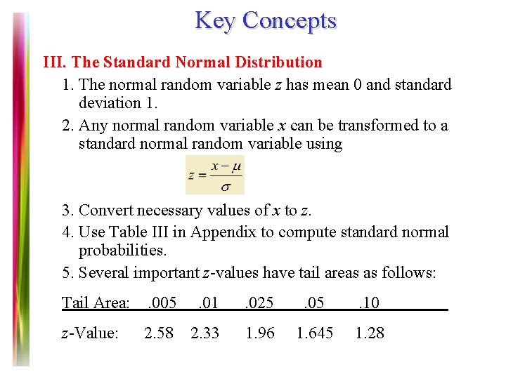
Key Concepts III. The Standard Normal Distribution 1. The normal random variable z has mean 0 and standard deviation 1. 2. Any normal random variable x can be transformed to a standard normal random variable using 3. Convert necessary values of x to z. 4. Use Table III in Appendix to compute standard normal probabilities. 5. Several important z-values have tail areas as follows: Tail Area: . 005 . 01 . 025 . 05 . 10 z-Value: 2. 58 2. 33 1. 96 1. 645 1. 28 Note 7 of 5 E

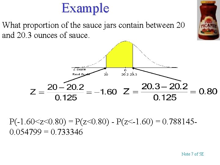
Example What proportion of the sauce jars contain between 20 and 20. 3 ounces of sauce. P(-1. 60<z<0. 80) = P(z<0. 80) - P(z<-1. 60) = 0. 7881450. 054799 = 0. 733346 Note 7 of 5 E

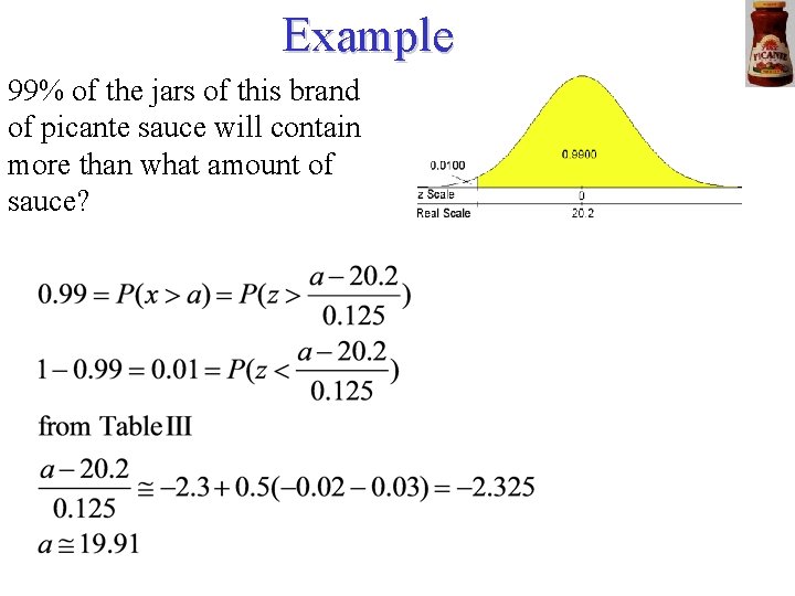
Example 99% of the jars of this brand of picante sauce will contain more than what amount of sauce? Note 7 of 5 E