ECE 1747 Parallel Programming Machineindependent Performance Optimization Techniques

ECE 1747 Parallel Programming Machine-independent Performance Optimization Techniques

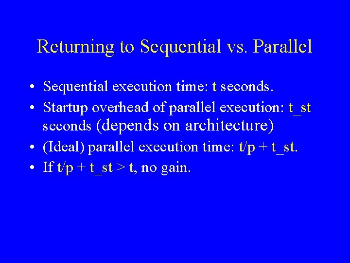
Returning to Sequential vs. Parallel • Sequential execution time: t seconds. • Startup overhead of parallel execution: t_st seconds (depends on architecture) • (Ideal) parallel execution time: t/p + t_st. • If t/p + t_st > t, no gain.

General Idea • Parallelism limited by dependences. • Restructure code to eliminate or reduce dependences. • Sometimes possible by compiler, but good to know how to do it by hand.

Example 1 for( i=0; i<n; i++ ) { tmp = a[i]; a[i] = b[i]; b[i] = tmp; } • Dependence on tmp.

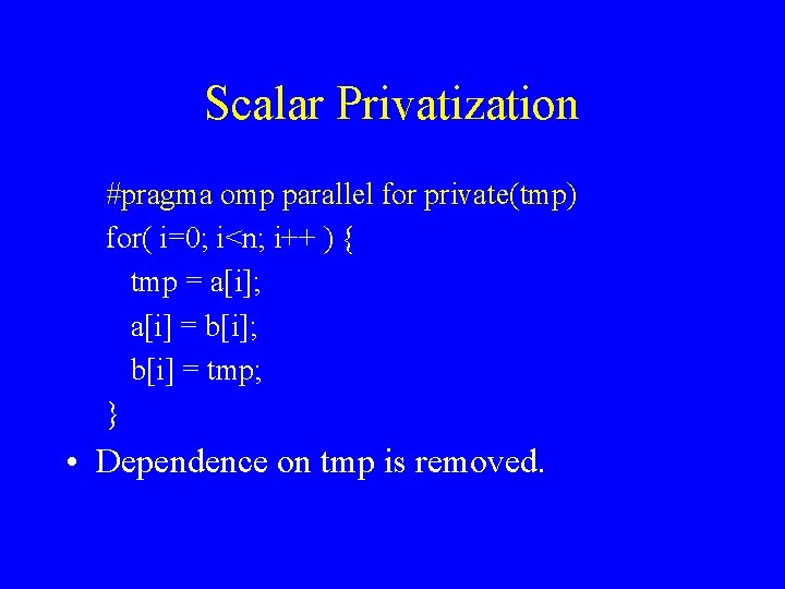
Scalar Privatization #pragma omp parallel for private(tmp) for( i=0; i<n; i++ ) { tmp = a[i]; a[i] = b[i]; b[i] = tmp; } • Dependence on tmp is removed.

Example 2 for( i=0, sum=0; i<n; i++ ) sum += a[i]; • Dependence on sum.

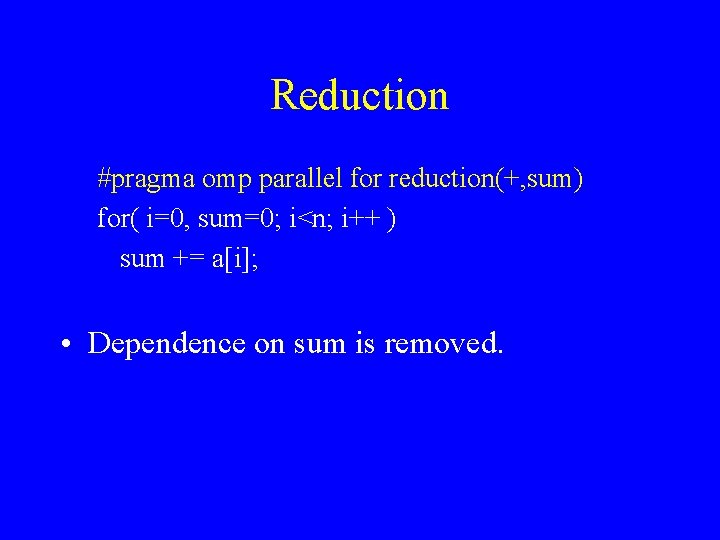
Reduction #pragma omp parallel for reduction(+, sum) for( i=0, sum=0; i<n; i++ ) sum += a[i]; • Dependence on sum is removed.

Example 3 for( i=0, index=0; i<n; i++ ) { index += i; a[i] = b[index]; } • Dependence on index. • Induction variable: can be computed from loop variable.

Induction Variable Elimination #pragma omp parallel for( i=0, index=0; i<n; i++ ) { a[i] = b[i*(i+1)/2]; } • Dependence removed by computing the induction variable.

Example 4 for( i=0, index=0; i<n; i++ ) { index += f(i); b[i] = g(a[index]); } • Dependence on induction variable index, but no closed formula for its value.

Loop Splitting for( i=0; i<n; i++ ) { index[i] += f(i); } #pragma omp parallel for( i=0; i<n; i++ ) { b[i] = g(a[index[i]]); } • Loop splitting has removed dependence.

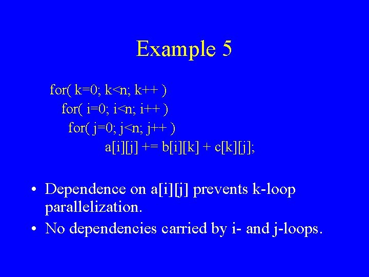
Example 5 for( k=0; k<n; k++ ) for( i=0; i<n; i++ ) for( j=0; j<n; j++ ) a[i][j] += b[i][k] + c[k][j]; • Dependence on a[i][j] prevents k-loop parallelization. • No dependencies carried by i- and j-loops.

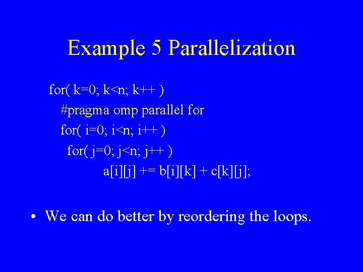
Example 5 Parallelization for( k=0; k<n; k++ ) #pragma omp parallel for( i=0; i<n; i++ ) for( j=0; j<n; j++ ) a[i][j] += b[i][k] + c[k][j]; • We can do better by reordering the loops.

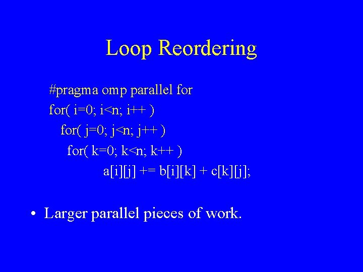
Loop Reordering #pragma omp parallel for( i=0; i<n; i++ ) for( j=0; j<n; j++ ) for( k=0; k<n; k++ ) a[i][j] += b[i][k] + c[k][j]; • Larger parallel pieces of work.

Example 6 #pragma omp parallel for(i=0; i<n; i++ ) a[i] = b[i]; #pragma omp parallel for( i=0; i<n; i++ ) c[i] = b[i]^2; • Make two parallel loops into one.

Loop Fusion #pragma omp parallel for(i=0; i<n; i++ ) { a[i] = b[i]; c[i] = b[i]^2; } • Reduces loop startup overhead.

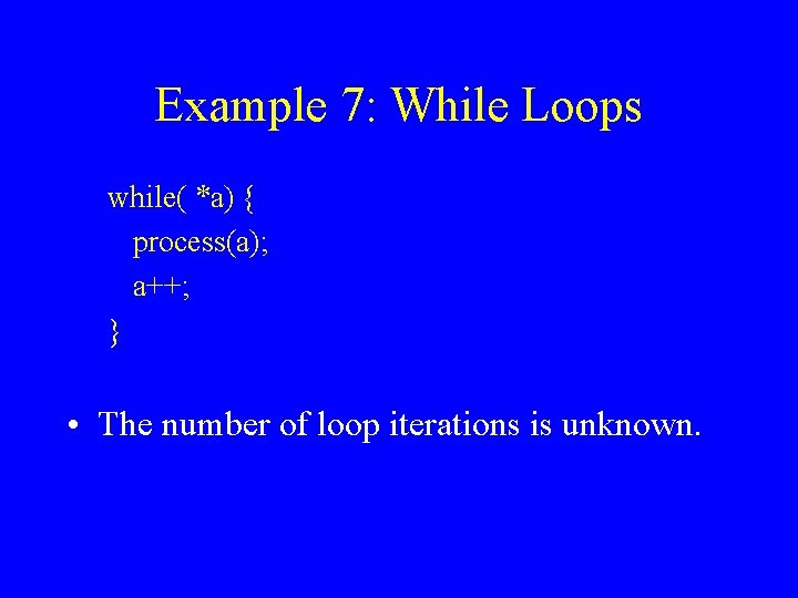
Example 7: While Loops while( *a) { process(a); a++; } • The number of loop iterations is unknown.

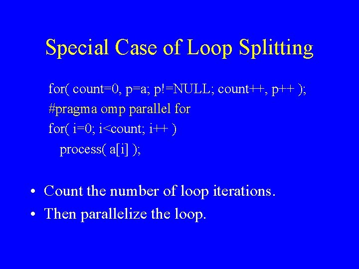
Special Case of Loop Splitting for( count=0, p=a; p!=NULL; count++, p++ ); #pragma omp parallel for( i=0; i<count; i++ ) process( a[i] ); • Count the number of loop iterations. • Then parallelize the loop.

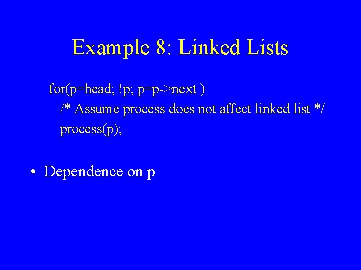
Example 8: Linked Lists for(p=head; !p; p=p->next ) /* Assume process does not affect linked list */ process(p); • Dependence on p

Another Special Case of Loop Splitting for( p=head, count=0; p!=NULL; p=p->next, count++); count[i] = f(count, omp_get_numthreads()); start[0] = head; for( i=0; i< omp_get_numthreads(); i++ ) { for( p=start[i], cnt=0; cnt<count[i]; p=p->next); start[i+1] = p->next; }

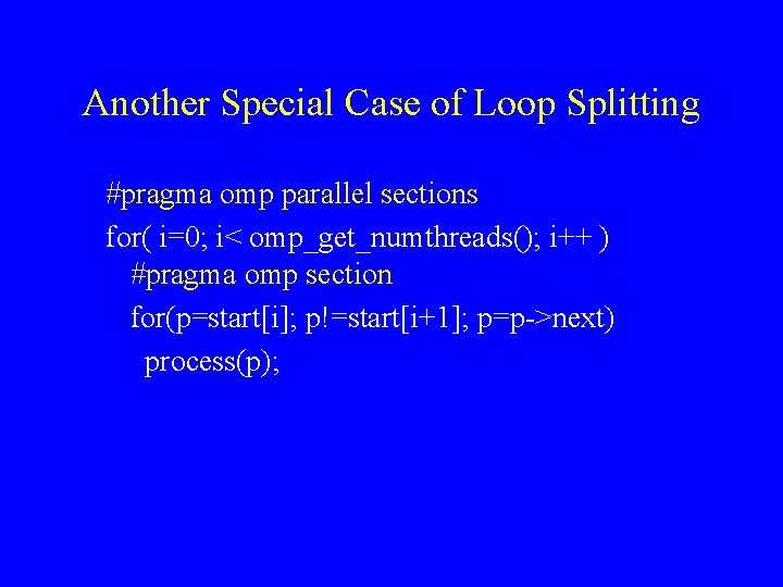
Another Special Case of Loop Splitting #pragma omp parallel sections for( i=0; i< omp_get_numthreads(); i++ ) #pragma omp section for(p=start[i]; p!=start[i+1]; p=p->next) process(p);

Example 9 for( i=0, wrap=n; i<n; i++ ) { b[i] = a[i] + a[wrap]; wrap = i; } • Dependence on wrap. • Only first iteration causes dependence.

Loop Peeling b[0] = a[0] + a[n]; #pragma omp parallel for( i=1; i<n; i++ ) { b[i] = a[i] + a[i-1]; }

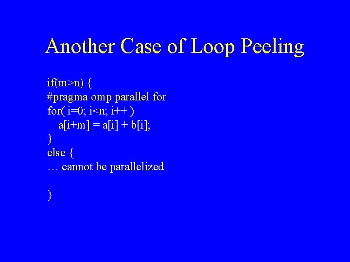
Example 10 for( i=0; i<n; i++ ) a[i+m] = a[i] + b[i]; • Dependence if m<n.

Another Case of Loop Peeling if(m>n) { #pragma omp parallel for( i=0; i<n; i++ ) a[i+m] = a[i] + b[i]; } else { … cannot be parallelized }

Summary • Reorganize code such that – dependences are removed or reduced – large pieces of parallel work emerge – loop bounds become known –… • Code can become messy … there is a point of diminishing returns.

Factors that Determine Speedup • Characteristics of parallel code – granularity – load balance – locality – communication and synchronization

Granularity • Granularity = size of the program unit that is executed by a single processor. • May be a single loop iteration, a set of loop iterations, etc. • Fine granularity leads to: – (positive) ability to use lots of processors – (positive) finer-grain load balancing – (negative) increased overhead

Granularity and Critical Sections • Small granularity => more processors => more critical section accesses => more contention.

Issues in Performance of Parallel Parts • • Granularity. Load balance. Locality. Synchronization and communication.

Load Balance • Load imbalance = different in execution time between processors between barriers. • Execution time may not be predictable. – Regular data parallel: yes. – Irregular data parallel or pipeline: perhaps. – Task queue: no.

Static vs. Dynamic • Static: done once, by the programmer – block, cyclic, etc. – fine for regular data parallel • Dynamic: done at runtime – task queue – fine for unpredictable execution times – usually high overhead • Semi-static: done once, at run-time

Choice is not inherent • MM or SOR could be done using task queues: put all iterations in a queue. – In heterogeneous environment. – In multitasked environment. • TSP could be done using static partitioning: give length-1 path to all processors. – If we did exhaustive search.

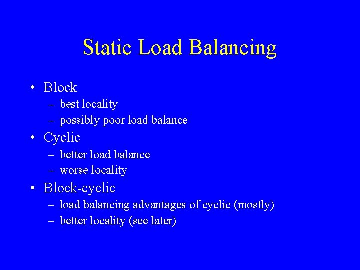
Static Load Balancing • Block – best locality – possibly poor load balance • Cyclic – better load balance – worse locality • Block-cyclic – load balancing advantages of cyclic (mostly) – better locality (see later)

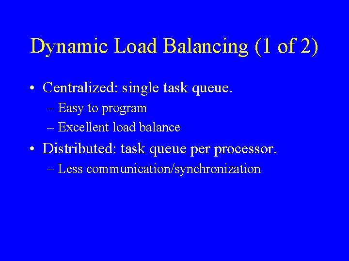
Dynamic Load Balancing (1 of 2) • Centralized: single task queue. – Easy to program – Excellent load balance • Distributed: task queue per processor. – Less communication/synchronization

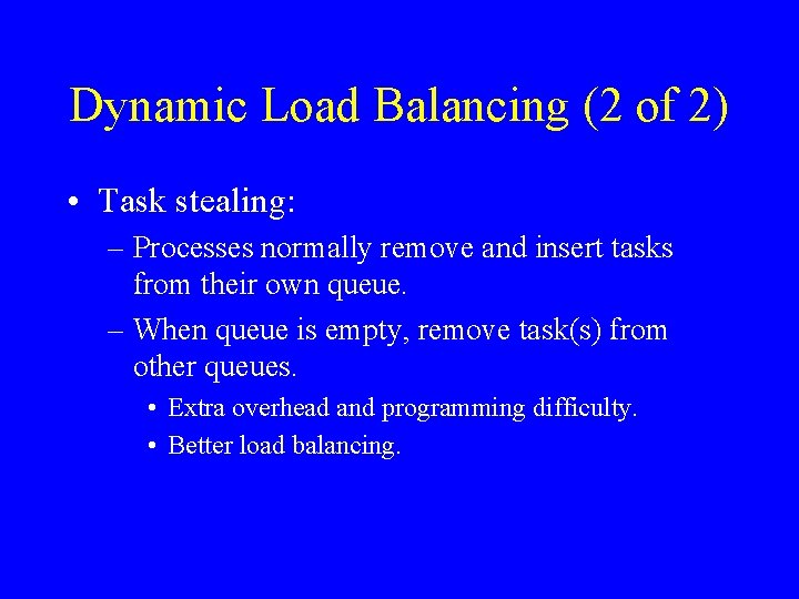
Dynamic Load Balancing (2 of 2) • Task stealing: – Processes normally remove and insert tasks from their own queue. – When queue is empty, remove task(s) from other queues. • Extra overhead and programming difficulty. • Better load balancing.

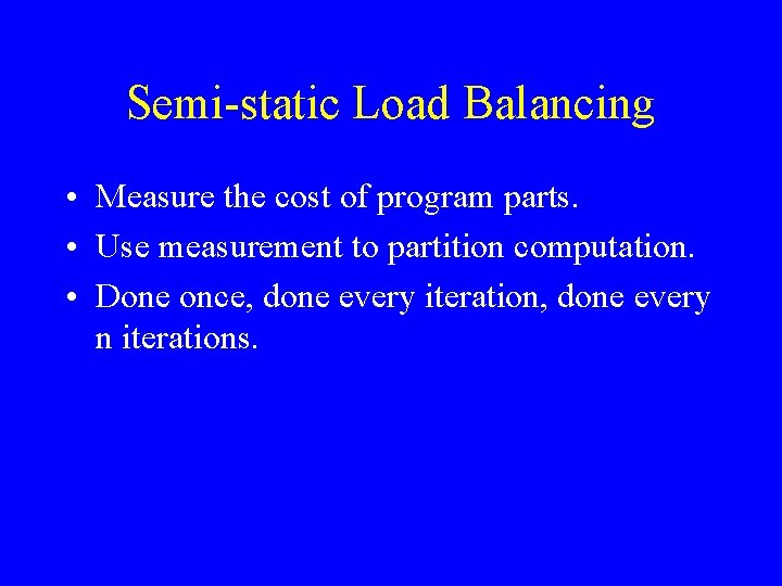
Semi-static Load Balancing • Measure the cost of program parts. • Use measurement to partition computation. • Done once, done every iteration, done every n iterations.

Molecular Dynamics (MD) • Simulation of a set of bodies under the influence of physical laws. • Atoms, molecules, celestial bodies, . . . • Have same basic structure.

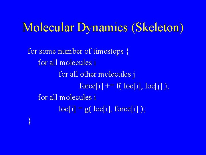
Molecular Dynamics (Skeleton) for some number of timesteps { for all molecules i for all other molecules j force[i] += f( loc[i], loc[j] ); for all molecules i loc[i] = g( loc[i], force[i] ); }

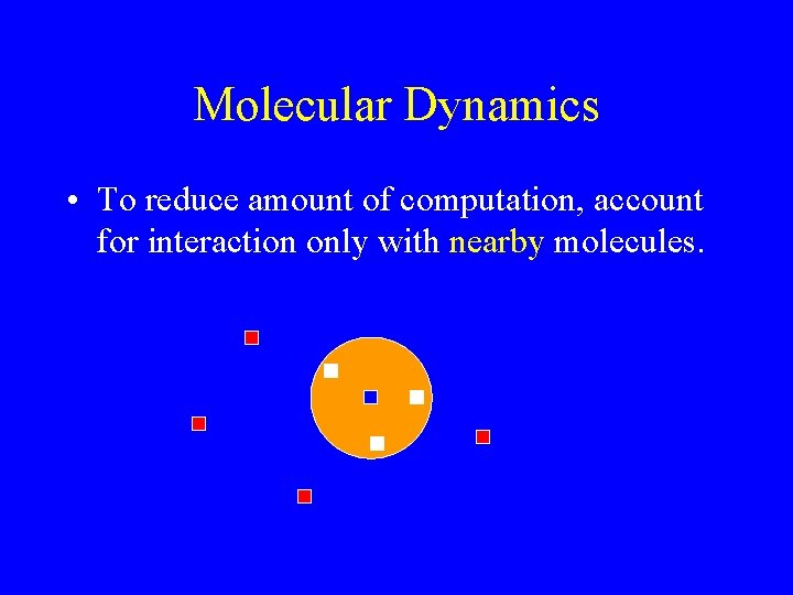
Molecular Dynamics • To reduce amount of computation, account for interaction only with nearby molecules.

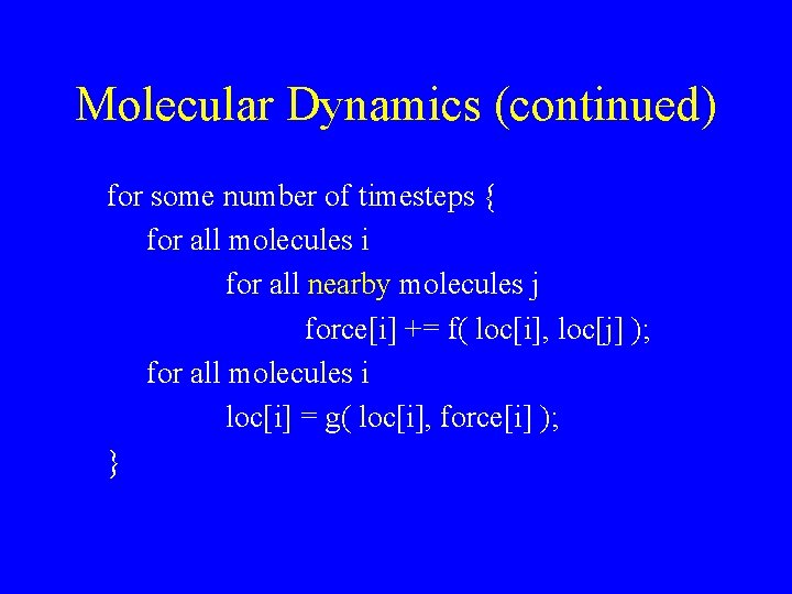
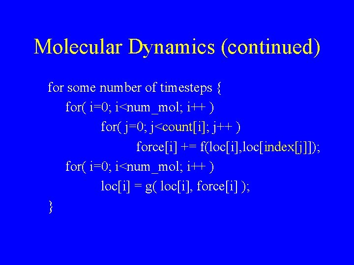
Molecular Dynamics (continued) for some number of timesteps { for all molecules i for all nearby molecules j force[i] += f( loc[i], loc[j] ); for all molecules i loc[i] = g( loc[i], force[i] ); }

Molecular Dynamics (continued) for each molecule i number of nearby molecules count[i] array of indices of nearby molecules index[j] ( 0 <= j < count[i])

Molecular Dynamics (continued) for some number of timesteps { for( i=0; i<num_mol; i++ ) for( j=0; j<count[i]; j++ ) force[i] += f(loc[i], loc[index[j]]); for( i=0; i<num_mol; i++ ) loc[i] = g( loc[i], force[i] ); }

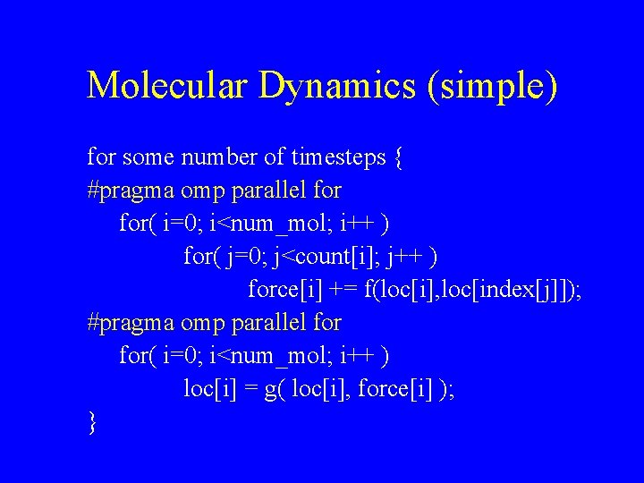
Molecular Dynamics (simple) for some number of timesteps { #pragma omp parallel for( i=0; i<num_mol; i++ ) for( j=0; j<count[i]; j++ ) force[i] += f(loc[i], loc[index[j]]); #pragma omp parallel for( i=0; i<num_mol; i++ ) loc[i] = g( loc[i], force[i] ); }

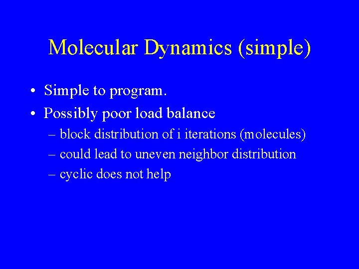
Molecular Dynamics (simple) • Simple to program. • Possibly poor load balance – block distribution of i iterations (molecules) – could lead to uneven neighbor distribution – cyclic does not help

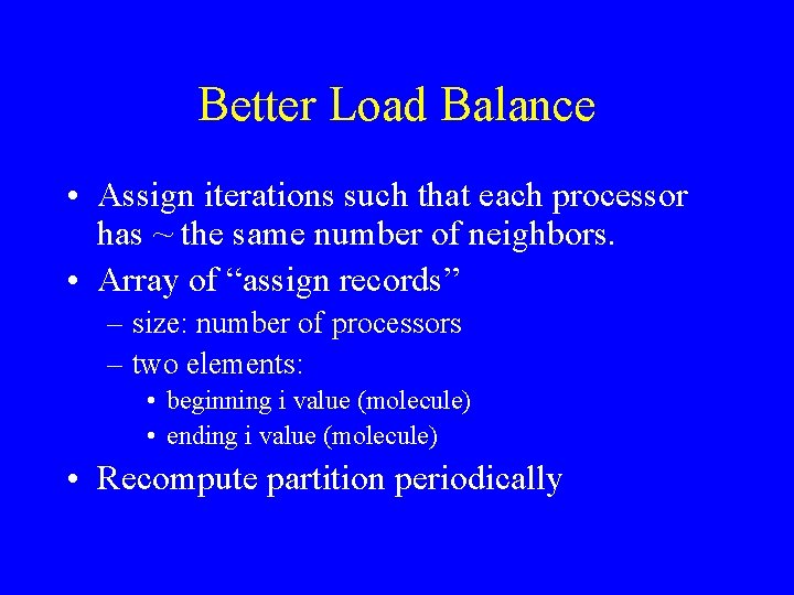
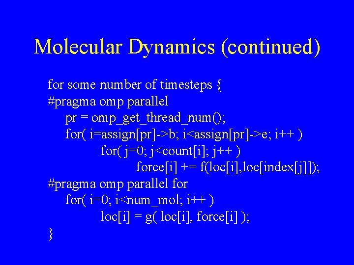
Better Load Balance • Assign iterations such that each processor has ~ the same number of neighbors. • Array of “assign records” – size: number of processors – two elements: • beginning i value (molecule) • ending i value (molecule) • Recompute partition periodically

Molecular Dynamics (continued) for some number of timesteps { #pragma omp parallel pr = omp_get_thread_num(); for( i=assign[pr]->b; i<assign[pr]->e; i++ ) for( j=0; j<count[i]; j++ ) force[i] += f(loc[i], loc[index[j]]); #pragma omp parallel for( i=0; i<num_mol; i++ ) loc[i] = g( loc[i], force[i] ); }

Frequency of Balancing • Every time neighbor list is recomputed. – once during initialization. – every iteration. – every n iterations. • Extra overhead vs. better approximation and better load balance.

Summary • Parallel code optimization – Critical section accesses. – Granularity. – Load balance.

Factors that Determine Speedup – granularity – load balancing – locality • uniprocessor • multiprocessor – synchronization and communication

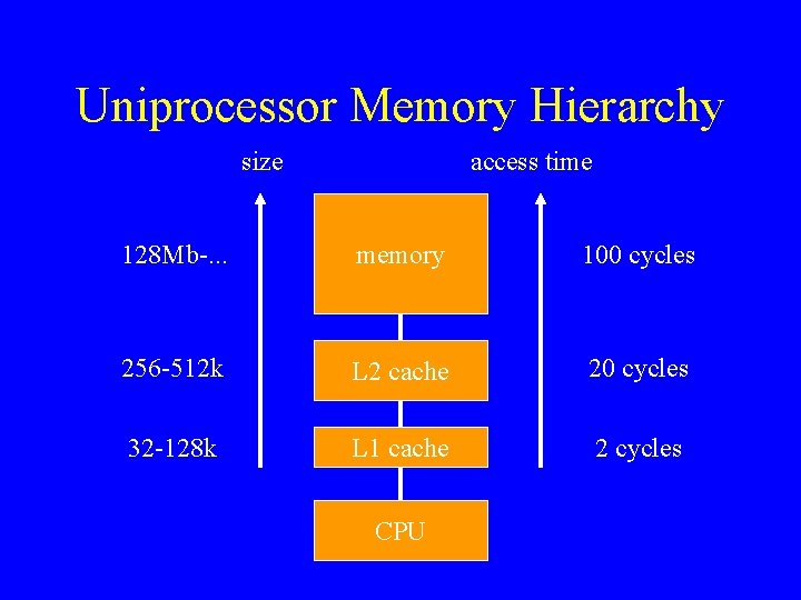
Uniprocessor Memory Hierarchy size access time 128 Mb-. . . memory 100 cycles 256 -512 k L 2 cache 20 cycles 32 -128 k L 1 cache 2 cycles CPU

Uniprocessor Memory Hierarchy • Transparent to user/compiler/CPU. • Except for performance, of course.

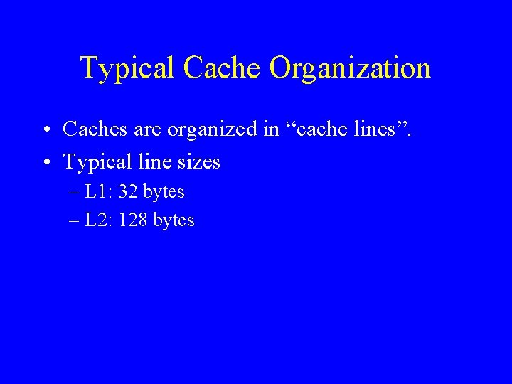
Typical Cache Organization • Caches are organized in “cache lines”. • Typical line sizes – L 1: 32 bytes – L 2: 128 bytes

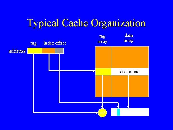
Typical Cache Organization tag index offset tag array data array address cache line =?

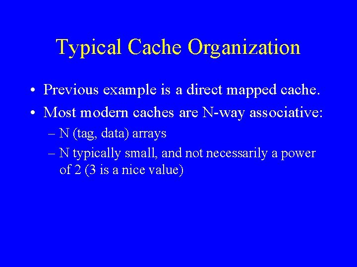
Typical Cache Organization • Previous example is a direct mapped cache. • Most modern caches are N-way associative: – N (tag, data) arrays – N typically small, and not necessarily a power of 2 (3 is a nice value)

Cache Replacement • If you hit in the cache, done. • If you miss in the cache, – Fetch line from next level in hierarchy. – Replace the current line at that index. – If associative, then choose a line within that set Various policies: e. g. , least-recently-used

Bottom Line • To get good performance, – You have to have a high hit rate. – You have to continue to access the data “close” to the data that you accessed recently.

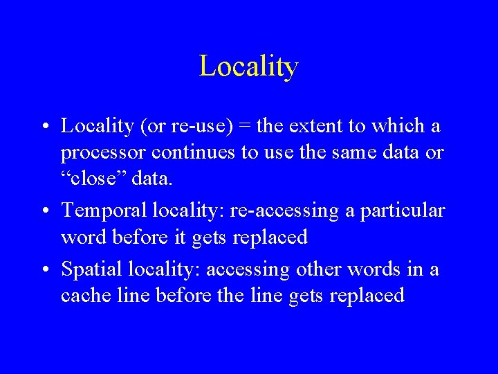
Locality • Locality (or re-use) = the extent to which a processor continues to use the same data or “close” data. • Temporal locality: re-accessing a particular word before it gets replaced • Spatial locality: accessing other words in a cache line before the line gets replaced

Example 1 for( i=0; i<n; i++ ) for( j=0; j<n; j++ ) grid[i][j] = temp[i][j]; • Good spatial locality in grid and temp (arrays in C laid out in row-major order). • No temporal locality.

Example 2 for( j=0; j<n; j++ ) for( i=0; i<n; i++ ) grid[i][j] = temp[i][j]; • No spatial locality in grid and temp. • No temporal locality.

Example 3 for( i=0; i<n; i++ ) for( j=0; j<n; j++ ) temp[i][j] = 0. 25 * (grid[i+1][j]+ grid[i][j-1]+grid[i][j+1]); • Spatial locality in temp. • Spatial locality in grid. • Temporal locality in grid?

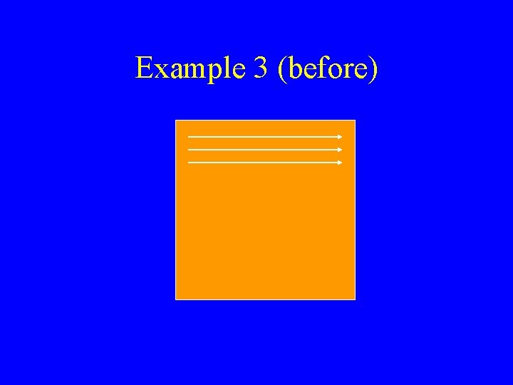
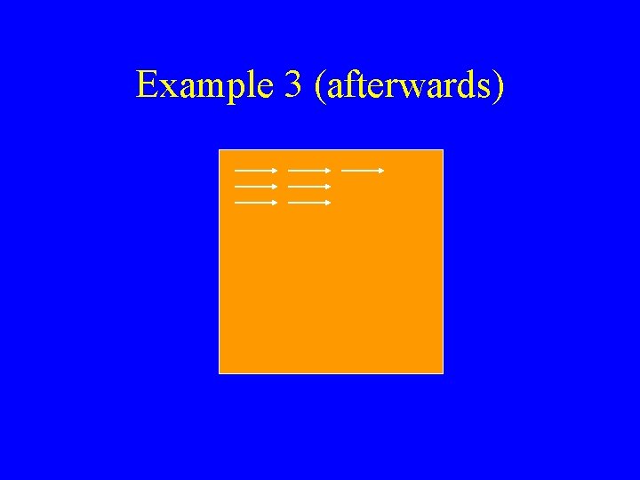
Access to grid[i][j] • First time grid[i][j] is used: temp[i-1, j]. • Second time grid[i][j] is used: temp[i, j-1]. • Between those times, 3 rows go through the cache. • If 3 rows > cache size, cache miss on second access.

Fix • Traverse the array in blocks, rather than row -wise sweep. • Make sure grid[i][j] still in cache on second access.

Example 3 (before)

Example 3 (afterwards)

Achieving Better Locality • • Technique is known as blocking / tiling. Compiler algorithms known. Few commercial compilers do it. Learn to do it yourself.

Locality in Parallel Programming • View parallel machine – not only as a multi-CPU system – but also as a multi-memory system

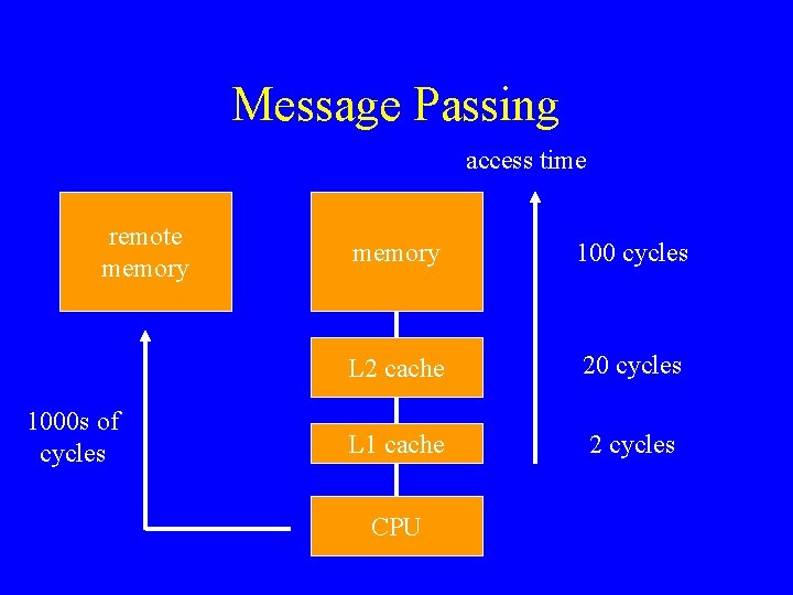
Message Passing access time remote memory 1000 s of cycles memory 100 cycles L 2 cache 20 cycles L 1 cache 2 cycles CPU

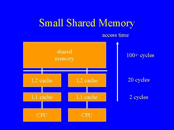
Small Shared Memory access time shared memory 100+ cycles L 2 cache 20 cycles L 1 cache 2 cycles CPU

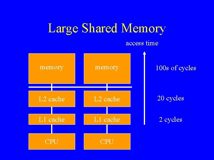
Large Shared Memory access time memory 100 s of cycles L 2 cache 20 cycles L 1 cache 2 cycles CPU

Note on Parallel Memory Hierarchies • In shared memory (small or large), memory hierarchy is transparent. • In message passing, memory hierarchy is not transparent -- managed by user. • Principle remains (largely) the same. • Transparent memory hierarchy can lead to unexpected locality loss in shared memory.

Locality in Parallel Programming • Is even more important than in sequential programming, because the memory latencies are longer.

Returning to Sequential vs. Parallel • A piece of code may be better executed sequentially if considered by itself. • But locality make it profitable to execute it in parallel. • Typically happens with initializations.

Example: Parallelization Ignoring Locality for( i=0; i<n; i++ ) a[i] = i; #pragma omp parallel for( i=0; i<n; i++ ) /* assume f is a very expensive function */ b[i] = f( a[i-1], a[i] );

Example: Taking Locality into Account #pragma omp parallel for( i=0; i<n; i++ ) a[i] = i; #pragma omp parallel for( i=0; i<n; i++ ) /* assume f is a very expensive function */ b[i] = f( a[i-1], a[i] )

How to Get Started? • First thing: figure what takes the time in your sequential program => profile it (gprof) ! • Typically, few parts (few loops) take the bulk of the time. • Parallelize those parts first, worrying about granularity and load balance. • Advantage of shared memory: you can do that incrementally. • Then worry about locality.

Performance and Architecture • Understanding the performance of a parallel program often requires an understanding of the underlying architecture. • There are two principal architectures: – distributed memory machines – shared memory machines • Microarchitecture plays a role too!