Stochastic Network Optimization tutorial M J Neely University

Stochastic Network Optimization (tutorial) M. J. Neely University of Southern California See detailed derivations for these results in: M. J. Neely, Stochastic Network Optimization with Application to Communication and Queueing Systems, Morgan & Claypool 2010. http: //www-bcf. usc. edu/~mjneely/

Outline • Queue Stability • Randomized Algs and Linear Programs for Queue Stability (known statistics) • Dynamic Algs and Drift-Plus-Penalty (unknown statistics) • Backpressure Examples (if time)

Queue Dynamics a(t) Q(t) b(t) Q(t+1) = max[Q(t) + a(t) – b(t), 0] or Q(t+1) = max[Q(t) + y(t), 0] where y(t) = a(t) – b(t) Note: Departures(t) = min[Q(t), b(t)]

Rate Stability a(t) Q(t) b(t) Definition: Q(t) is rate stable if: limt ∞ Q(t)/t = 0 (with probability 1) Why use this definition?

Rate Stability Theorem a(t) b(t) Q(t) Theorem: Recall y(t) = a(t) – b(t). Suppose: t-1 limt ∞ (1/t)∑τ=0 y(τ) = yav (w. p. 1) Then Q(t) is rate stable if and only if: yav ≤ 0 Proof: Necessary condition is straightforward. Sufficient condition requires a trick.

Example Arrival Processes a(t) with Time Average Rate λ • Deterministic: 1 packet periodically arrives every 10 slots. t-1 limt ∞ (1/t)∑τ=0 a(τ) = 1/10 (w. p. 1) • Random: {a(t)} i. i. d. over t in {0, 1, 2, …}. t-1 limt ∞ (1/t)∑τ=0 a(τ) = E{a(0)} (w. p. 1)

Outline • Queue Stability • Randomized Algs and Linear Programs for Queue Stability (known statistics) • Dynamic Algs and Drift-Plus-Penalty (unknown statistics) • Backpressure Examples (if time)

Scheduling for Queue Stability Arrival rate λ 1 Q 1(t) b 1(t) Arrival rate λK QK(t) b. K(t) If we make service allocations every slot to ensure that each bi(t) has time average bi, av , and: then by the rate stability theorem, all queues are rate stable.

Scheduling for Queue Stability Arrival rate λ 1 Q 1(t) b 1(t) Arrival rate λK QK(t) b. K(t) If we make service allocations every slot to ensure that each bi(t) has time average bi, av , and: bi, av ≥ λi for all i in {1, …, K} then by the rate stability theorem, all queues are rate stable.

A 3 -Queue, 2 -Server System: λ 1 Q 1(t) λ 2 Q 2(t) λ 3 Q 3(t) A server can serve 1 packet/slot. Every slot, choose: (b 1(t), b 2(t), b 3(t)) in {(1, 1, 0), (1, 0, 1), (0, 1, 1)} How to schedule the servers to make all queues rate stable?

Exercise (apply what we just learned): λ 1 λ 2 λ 3 1 2 3 Design a stabilizing server allocation algorithm for: (a) (λ 1, λ 2, λ 3) = (1, 1/2). (b) (λ 1, λ 2, λ 3) = (2/3, 2/3). (c) (λ 1, λ 2, λ 3) = (1/2, 3/4). (d) (λ 1, λ 2, λ 3) = (0. 4, 0. 7, 0. 8). (e) (λ 1, λ 2, λ 3) = (0. 46, 0. 82, 0. 70). How many can you do in 5 minutes? (a) and (b) are easy.

LP Approach to part (e): λ 1 λ 2 λ 3 1 2 3 Choose i. i. d. with dist: p 1 = Pr[choose (1, 1, 0)] p 2 = Pr[choose (1, 0, 1)] p 3 = Pr[choose (0, 1, 1)] Want to support (λ 1, λ 2, λ 3) = (0. 46, 0. 82, 0. 70). (1) (0) (0. 46) p 1 (1) + p 2 (0) + p 3 (1) ≥ (0. 82) (0) (1) (0. 70) p 1 + p 2 + p 3 = 1 p 1≥ 0, p 2≥ 0, p 3≥ 0 Linear Program

General Problem (no channel state variation) λ 1 1 b 1(t) λK K b. K(t) Choose b(t)= (b 1(t), …, b. K(t)) in General set Γ Γ = {b(1), b(2) , b(3) , … , b(M-1) , b(M) } Choose i. i. d. with distribution given by LP: M ∑m=1 b(m)p(m) ≥ λ (where λ= (λ 1, . . . , λK) ) p(m) ≥ 0 for all m in {1, …, M} M ∑m=1 p(m) = 1 Note: We cannot do better than this! This provably defines the capacity region!

General Problem (no channel state variation) λ 1 1 b 1(t) λK K b. K(t) Choose b(t)= (b 1(t), …, b. K(t)) in General set Γ Γ = {b(1), b(2) , b(3) , … , b(M-1) , b(M) } Equivalently: Design a randomized alg that chooses b(t) i. i. d. over slots so that: E[b(t)] ≥ λ Note: We cannot do better than this! This provably defines the capacity region!

General Problem (with channel state variation) ω(t) = random states (i. i. d. every slot) with distribution π(ω) = Pr[ω(t)=ω] α(t) = control action (chosen in action space Aω(t) ) Penalties yi(t) = yi(α(t), ω(t)). Minimize: y 0 Subject to: (1) yi ≤ 0 for all i in {1, . . , K} (2) α(t) in Aω(t) for all slots t.

LP Solution for known π(ω) = Pr[ω(t)=ω] Minimize: y 0 Subject to: (1) yi ≤ 0 for all i in {1, . . , K} (2) α(t) in Aω(t) for all slots t. For simplicity of this slide, assume finite sets: ω(t) in {ω1, ω2, …, ωJ} , α(t) in {α 1, α 2, …, αΜ} Recall that yi(t) = yi(α(t), ω(t)). Let p(αm , ωj) = Pr[Choose α(t) = αm | ω(t) =ωj] Exercise: Write an LP to solve this. Start with: Minimize: J M ∑j=1∑m=1 π(ωj) p(αm, ωj) y 0(αm, ωj)

LP Solution for known π(ω) = Pr[ω(t)=ω] Minimize: y 0 Subject to: (1) yi ≤ 0 for all i in {1, . . , K} (2) α(t) in Aω(t) for all slots t. For simplicity of this slide, assume finite sets: ω(t) in {ω1, ω2, …, ωJ} , α(t) in {α 1, α 2, …, αΜ} Recall that yi(t) = yi(α(t), ω(t)). Let p(αm , ωj) = Pr[Choose α(t) = αm | ω(t) =ωj] Equivalently: Use randomized alg with: Min: E{y 0(t)} Subject to: E{yi(t)} ≤ 0 for all i in {1, …, K}

Properties of the LP Known Constants: • π(ω) for all ω in {ω1, ω2, …, ωJ}. (J is typically exponential in network size) • yi(αm, ωj) for all i, m, j in {1, …, K}x{1, …. M}x{1, …, J} LP Variables: • p(αm, ωj) for all m in {1, …, M}, j in {1, …, J}. (number of variables is typically exponential in network size)

Disadvantages of this LP Approach? • • . .

Disadvantages of this LP Approach • Problem is huge. - Non-polynomial number of variables. • Need to know distribution π(ω). -Typically non-polynomial number of ω. -Good estimate would take “years”of samples. -Probabilities will certainly change by this time. • Not Adaptive to Changes. • What if ω(t) is non-i. i. d. ? Non-ergodic? • For queueing networks: -Delay guarantees? -Flow control?

Outline • Queue Stability • Randomized Algs and Linear Programs for Queue Stability (known statistics) • Dynamic Algs and Drift-Plus-Penalty (unknown statistics) • Backpressure Examples (if time)

Dynamic Approach Minimize: y 0 Subject to: (1) yi ≤ 0 for all i in {1, . . , K} (2) α(t) in Aω(t) for all slots t. (1) Make “virtual queue” for each inequality constraint: Qi(t+1) = max[Qi(t) + yi(t), 0] for i in {1, …, K} Why? Because: Qi(t)/t 0 implies yi ≤ 0

Virtual Queue Stability Theorem: Recall: Qi(t+1) = max[Qi(t) + yi(t), 0] Theorem: Qi(t)/t 0 implies yi ≤ 0. Proof: Qi(τ+1) = max[Qi(τ) + yi(τ), 0] ≥ Qi(τ) + yi(τ). Thus: Qi(τ+1) - Qi(τ) ≥ yi(τ) for all τ. Use telescoping sums over τ in {0, …, t-1}: Qi(t) – Qi(0) ≥ ∑t-1 τ=0 yi(τ). Divide by t and take limit as t ∞.

Problem Becomes Minimize: y 0 Subject to: (1) Qi(t) stable for all i in {1, . . , K} (2) α(t) in Aω(t) for all slots t. (2) Define L(t) = sum of squares of queues (times ½): L(t) = (1/2)∑i. Qi(t)2 Why? Because if L(t) is “small, ” then all queues are “small. ” (3) Define the “drift” Δ(t): Δ(t) = L(t+1) – L(t)

Drift-Plus-Penalty Algorithm Minimize: y 0 Subject to: (1) Qi(t) stable for all i in {1, . . , K} (2) α(t) in Aω(t) for all slots t. (4) Every slot t, observe ω(t), Q(t). Then choose α(t) in Aω(t) to greedily minimize a bound on: Drift-Plus-Penalty: Δ(t) + Vy 0(α(t), ω(t)) (5) Update virtual queues for i in {1, …, K}: Qi(t+1) = max[Qi(t) + yi(α(t), ω(t)), 0]

Drift-Plus-Penalty Bound Recall: Qi(t+1) = max[Qi(t) + yi(α(t), ω(t)), 0]. Thus: Qi(t+1)2 ≤ [Qi(t) + yi(α(t), ω(t))]2 = Qi(t)2 + yi(α(t), ω(t)) 2 + 2 Qi(t)yi(α(t), ω(t)) Assuming squares of yi(α(t), ω(t)) 2 are bounded: Δ(t) ≤ B + ∑i. Qi(t)yi(α(t), ω(t)) So: Δ(t) + Vy 0(α(t), ω(t)) ≤ B + ∑i. Qi(t)yi(α(t), ω(t)) + Vy 0(α(t), ω(t))

Δ(t) + Vy 0(α(t), ω(t)) ≤ B + ∑i. Qi(t)yi(α(t), ω(t)) + Vy 0(α(t), ω(t)) The action is thus: Every slot t, observe ω(t), Q(t). Then choose α(t) by: Minimize: ∑i. Qi(t)yi(α(t), ω(t)) + Vy 0(α(t), ω(t)) Subject to: α(t) in Aω(t). • No knowledge of π(ω) required. • No curse of dimensionality. • Provably adapts to changes, general sample paths.

Performance Tradeoff Theorem: Assume ω(t) i. i. d. for simplicity: Theorem: For any V≥ 0. If the problem is feasible, then the drift-plus-penalty algorithm stabilizes all virtual queues. Further: (i) yi ≤ 0 for all i in {1, . . , K}. (ii) y 0 ≤ y 0 opt + B/V (iii) If there is an “interior point” of the feasibility region, then Qi ≤ O(V) for all i in {1, . . , K}.

Performance Tradeoff Theorem: Assume ω(t) i. i. d. for simplicity: Proof of (ii) [parts (i) and (iii) just as easy]: Δ(t) + Vy 0(α(t), ω(t)) ≤ B + ∑i. Qi(t)yi(α(t), ω(t)) + Vy 0(α(t), ω(t)) ≤ B + ∑i. Qi(t)yi(α*(t), ω(t)) + Vy 0(α*(t), ω(t)) For any other (possibly randomized) decision α*(t). Let’s re-write the above to give more room to work…

Performance Tradeoff Theorem: Assume ω(t) i. i. d. for simplicity: Proof of (ii) [continued]: Δ(t) + Vy 0(α(t), ω(t)) ≤ B + ∑i. Qi(t)yi(α*(t), ω(t)) + Vy 0(α*(t), ω(t)) For any other (possibly randomized) decision α*(t).

Performance Tradeoff Theorem: Assume ω(t) i. i. d. for simplicity: Proof of (ii) [continued]: Δ(t) + Vy 0(α(t), ω(t)) ≤ B + ∑i. Qi(t)yi(α*(t), ω(t)) + Vy 0(α*(t), ω(t)) For any other (possibly randomized) decision α*(t). Now use existence of randomized policy α*(t) that solves the problem: E[y 0(α*(t), ω(t))] = y 0 opt E[yi(α*(t), ω(t))] ≤ 0 for all i in {1, …, K} Now just take expectations…

Performance Tradeoff Theorem: Assume ω(t) i. i. d. for simplicity: Proof of (ii) [continued]: E[Δ(t) + Vy 0(α(t), ω(t))] ≤ B + E[∑i. Qi(t)yi(α*(t), ω(t))] + VE[y 0(α*(t), ω(t))] For any other (possibly randomized) decision α*(t). Now use existence of randomized policy α*(t) that solves the problem: E[y 0(α*(t), ω(t))] = y 0 opt E[yi(α*(t), ω(t))] ≤ 0 for all i in {1, …, K} Now just take expectations…

Performance Tradeoff Theorem: Assume ω(t) i. i. d. for simplicity: Proof of (ii) [continued]: 0 E[Δ(t) + Vy 0(α(t), ω(t))] ≤ B + E[∑i. Qi(t)yi(α*(t), ω(t))] + VE[y 0(α*(t), ω(t))] y For any other (possibly randomized) decision α*(t). opt 0 Now use existence of randomized policy α*(t) that solves the problem: E[y 0(α*(t), ω(t))] = y 0 opt E[yi(α*(t), ω(t))] ≤ 0 for all i in {1, …, K} Now just take expectations…

Performance Tradeoff Theorem: Assume ω(t) i. i. d. for simplicity: Proof of (ii) [continued]: E[Δ(t) + Vy 0(α(t), ω(t))] ≤ B + Vy 0 opt

Performance Tradeoff Theorem: Assume ω(t) i. i. d. for simplicity: Proof of (ii) [continued]: E[Δ(t) + Vy 0(α(t), ω(t))] ≤ B + Vy 0 opt Sum over t in {0, …, T-1}, divide by T: opt (1/T){ E[L(T)]–E[L(0)] + V∑T-1 E[y (α(t), ω(t))] } ≤ B+V y t=0 0 0 Thus (since L(T)≥ 0, L(0) =0): opt (1/T) ∑T-1 E[y (α(t), ω(t))] ≤ B/V + y t=0 0 0

Outline • Queue Stability • Randomized Algs and Linear Programs for Queue Stability (known statistics) • Dynamic Algs and Drift-Plus-Penalty (unknown statistics) • Backpressure Examples (if time)

Backpressure and Power Optimization for Multi-Hop Networks (An Application of “Drift-Plus-Penalty”) 2 1 5 4 6 1 3 2

6 μ 15=2 4 1 2 6 μ 45=1 3 5 1 4 (a) 6 4 5 (c) 3 5 μ 23=1 (b) 1 μ 45=1 2 μ 21=1 3 2 6 1 μ 32=1 μ 54=1 4 2 5 (d) 3

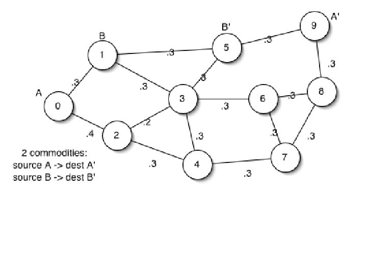
Diversity Backpressure Routing (DIVBAR) From: M. J. Neely and R. Urgaonkar, “Optimal Backpressure Routing in Wireless Networks with Multi-Receiver Diversity, ” Ad Hoc Networks (Elsevier), vol. 7, no. 5, pp. 862 -881, July 2009. (conference version in CISS 2006). • Multi-Hop Wireless Network with Probabilistic Channel Errors. • Multiple Neighbors can overhear same transmission, increasing the prob. of at least one successful reception (“multi-receiver diversity”). • Prior use of multi-receiver diversity: Routing heuristics: (SDF Larsson 2001)(Ge. Raf Zorzi, Rao 2003) (Ex. OR Biswas, Morris 2005). Sending one packet (DP): (Lott, Teneketzis 2006)(Javidi, Teneketzis 2004) (Laufer, Dubois-Ferriere, Kleinrock 2009). • Our backpressure approach (DIVBAR) gets max throughput, and can also minimize average power subject to network stability.

Cut capacity = 0. 9 packets/slot

Cut capacity = 0. 9 packets/slot • Network capacity: λΑ = λΒ = 0. 9/2 = 0. 45 • Max throughput of Ex. OR: λA = λΒ = (. 3 +. 7*. 3)/2 = 0. 255 *Note: The network capacity 0. 45 for this example was mistakenly stated as 0. 455 in [Neely, Urgaonkar 2009].

Ex. OR [Biswas, Morris 05] DIVBAR, E-DIVBAR [Neely, Urgaonkar 2009]

Ex. OR [Biswas, Morris 05] DIVBAR, E-DIVBAR [Neely, Urgaonkar 2009]

Ex. OR [Biswas, Morris 05] DIVBAR, E-DIVBAR [Neely, Urgaonkar 2009]

Ex. OR [Biswas, Morris 05] DIVBAR, E-DIVBAR [Neely, Urgaonkar 2009]

DIVBAR for Mobile Networks = Stationary Node = Locally Mobile Node = Fully Mobile Node = Sink

DIVBAR for Mobile Networks = Stationary Node = Locally Mobile Node = Fully Mobile Node = Sink

DIVBAR for Mobile Networks = Stationary Node = Locally Mobile Node = Fully Mobile Node = Sink

DIVBAR for Mobile Networks = Stationary Node = Locally Mobile Node = Fully Mobile Node = Sink

DIVBAR for Mobile Networks = Stationary Node = Locally Mobile Node = Fully Mobile Node = Sink

DIVBAR for Mobile Networks = Stationary Node = Locally Mobile Node = Fully Mobile Node = Sink

DIVBAR for Mobile Networks = Stationary Node = Locally Mobile Node = Fully Mobile Node = Sink

DIVBAR for Mobile Networks = Stationary Node = Locally Mobile Node = Fully Mobile Node = Sink

DIVBAR for Mobile Networks = Stationary Node = Locally Mobile Node = Fully Mobile Node = Sink

DIVBAR for Mobile Networks = Stationary Node = Locally Mobile Node = Fully Mobile Node = Sink

DIVBAR for Mobile Networks = Stationary Node = Locally Mobile Node = Fully Mobile Node = Sink

Average Total Backlog Versus Input rate for Mobile DIVBAR

Average Power Versus Delay (Fix a set of transmission rates for each node) Avg. Power Performance-Delay Tradeoff: [O(1/V), O(V)] Avg. Delay

Average Power Versus Delay (Fix a set of transmission rates for each node) Avg. Power Performance-Delay Tradeoff: [O(1/V), O(V)] Avg. Delay

Average Power Versus Delay (Fix a set of transmission rates for each node) Avg. Power Performance-Delay Tradeoff: [O(1/V), O(V)] Avg. Delay

Average Power Versus Delay (Fix a set of transmission rates for each node) Avg. Power Performance-Delay Tradeoff: [O(1/V), O(V)] Avg. Delay

Average Power Versus Delay (Fix a set of transmission rates for each node) Avg. Power Performance-Delay Tradeoff: [O(1/V), O(V)] Avg. Delay

Average Power Versus Delay (Fix a set of transmission rates for each node) Avg. Power Performance-Delay Tradeoff: [O(1/V), O(V)] Avg. Delay

Average Power Versus Delay (Fix a set of transmission rates for each node) Avg. Power Performance-Delay Tradeoff: [O(1/V), O(V)] Avg. Delay

Average Power Versus Delay (Fix a set of transmission rates for each node) Avg. Power Performance-Delay Tradeoff: [O(1/V), O(V)] Avg. Delay