MAMAS Computer Architecture Efficient Code Compiler Techniques and

MAMAS – Computer Architecture Efficient Code, Compiler Techniques and Optimizations Oren Katzengold and Dr. Avi Mendelson Some of the slides were taken from: (1) Jim Smith (2) Different sources from the NET Lecture 8 – Compiler Optimizations © Avi Mendelson, 5/2005 1

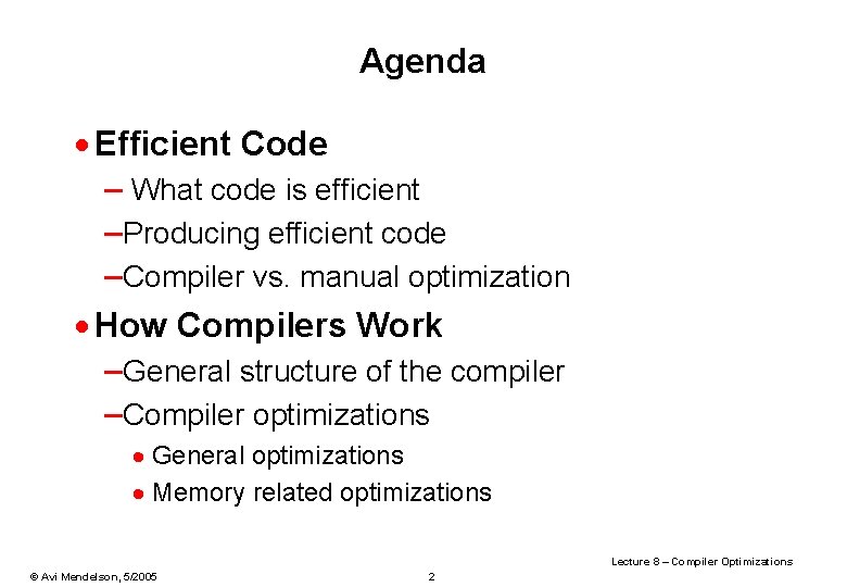
Agenda · Efficient Code – What code is efficient –Producing efficient code –Compiler vs. manual optimization · How Compilers Work –General structure of the compiler –Compiler optimizations · General optimizations · Memory related optimizations Lecture 8 – Compiler Optimizations © Avi Mendelson, 5/2005 2

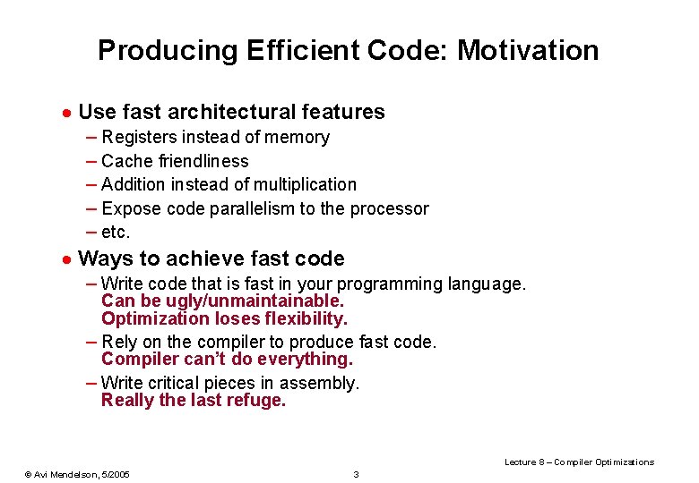
Producing Efficient Code: Motivation · Use fast architectural features – Registers instead of memory – Cache friendliness – Addition instead of multiplication – Expose code parallelism to the processor – etc. · Ways to achieve fast code – Write code that is fast in your programming language. Can be ugly/unmaintainable. Optimization loses flexibility. – Rely on the compiler to produce fast code. Compiler can’t do everything. – Write critical pieces in assembly. Really the last refuge. Lecture 8 – Compiler Optimizations © Avi Mendelson, 5/2005 3

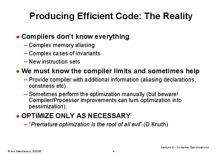
Producing Efficient Code: The Reality · Compilers don’t know everything – Complex memory aliasing – Complex cases of invariants – New instruction sets · We must know the compiler limits and sometimes help – Provide compiler with additional information (aliasing declarations, constness etc) – Sometimes perform the optimization manually (but beware! Compiler/Processor improvements can turn optimization into pessimization). · OPTIMIZE ONLY AS NECESSARY – “Premature optimization is the root of all evil” (D. Knuth) Lecture 8 – Compiler Optimizations © Avi Mendelson, 5/2005 4

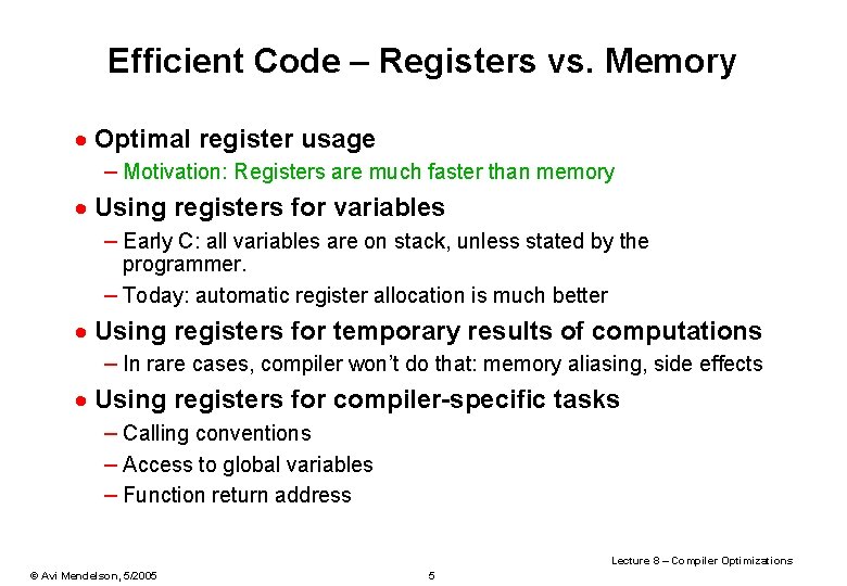
Efficient Code – Registers vs. Memory · Optimal register usage – Motivation: Registers are much faster than memory · Using registers for variables – Early C: all variables are on stack, unless stated by the programmer. – Today: automatic register allocation is much better · Using registers for temporary results of computations – In rare cases, compiler won’t do that: memory aliasing, side effects · Using registers for compiler-specific tasks – Calling conventions – Access to global variables – Function return address Lecture 8 – Compiler Optimizations © Avi Mendelson, 5/2005 5

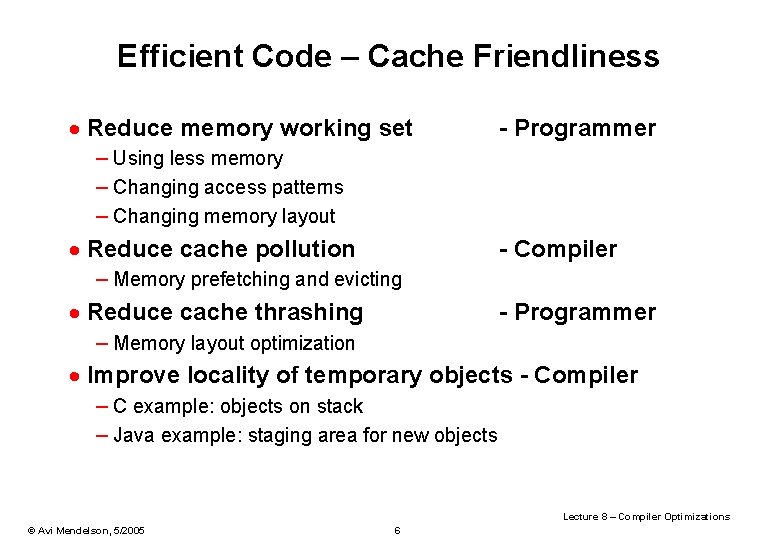
Efficient Code – Cache Friendliness · Reduce memory working set - Programmer – Using less memory – Changing access patterns – Changing memory layout · Reduce cache pollution - Compiler – Memory prefetching and evicting · Reduce cache thrashing - Programmer – Memory layout optimization · Improve locality of temporary objects - Compiler – C example: objects on stack – Java example: staging area for new objects Lecture 8 – Compiler Optimizations © Avi Mendelson, 5/2005 6

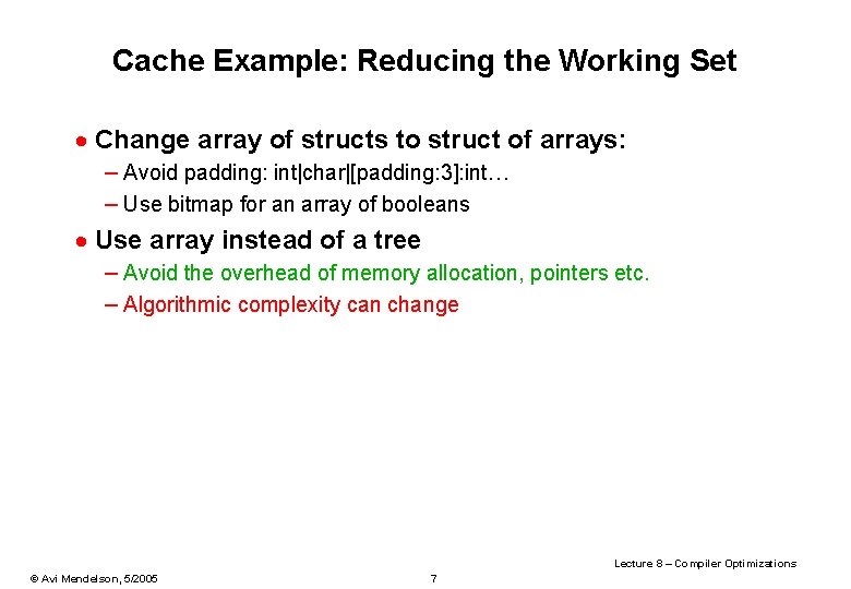
Cache Example: Reducing the Working Set · Change array of structs to struct of arrays: – Avoid padding: int|char|[padding: 3]: int… – Use bitmap for an array of booleans · Use array instead of a tree – Avoid the overhead of memory allocation, pointers etc. – Algorithmic complexity can change Lecture 8 – Compiler Optimizations © Avi Mendelson, 5/2005 7

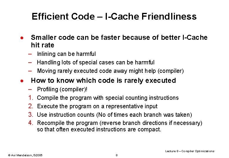
Efficient Code – I-Cache Friendliness · Smaller code can be faster because of better I-Cache hit rate – Inlining can be harmful – Handling lots of special cases can be harmful – Moving rarely executed code away might help (compiler) · How to know which code is rarely executed – 1. 2. 3. 4. Profiling (compiler)! Compile the program with special counting instructions Execute the program on a representative input Use instruction counts (No of times each branch was taken) Recompile the program (reverse branch directions if necessary) so that often executed instructions are compact. Lecture 8 – Compiler Optimizations © Avi Mendelson, 5/2005 8

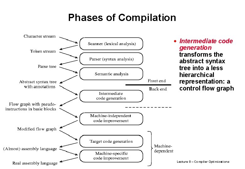
General structure of compiler Lecture 8 – Compiler Optimizations © Avi Mendelson, 5/2005 9

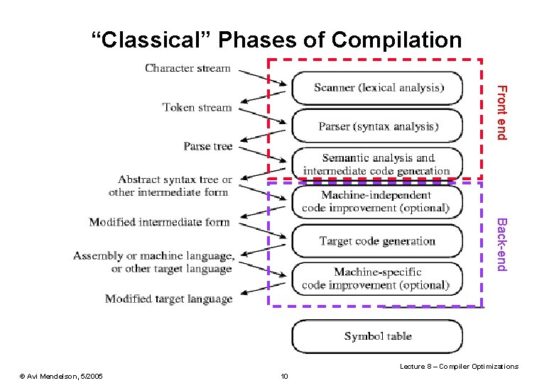
“Classical” Phases of Compilation Front end Back-end Lecture 8 – Compiler Optimizations © Avi Mendelson, 5/2005 10

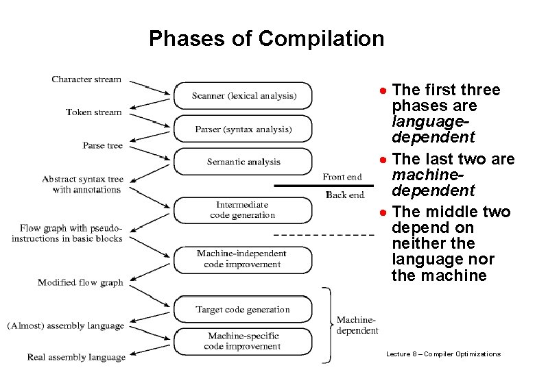
Phases of Compilation · The first three phases are languagedependent · The last two are machinedependent · The middle two depend on neither the language nor the machine Lecture 8 – Compiler Optimizations © Avi Mendelson, 5/2005 11

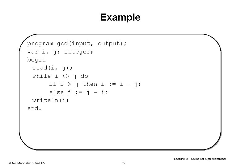
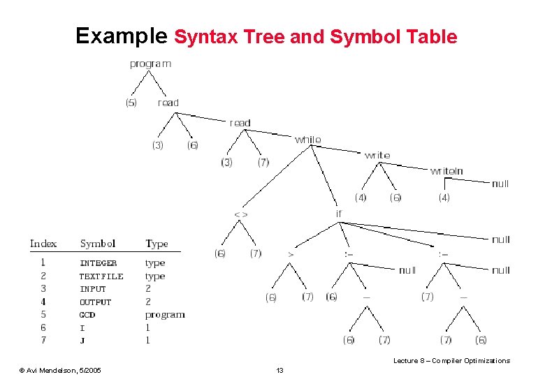
Example program gcd(input, output); var i, j: integer; begin read(i, j); while i <> j do if i > j then i : = i – j; else j : = j – i; writeln(i) end. Lecture 8 – Compiler Optimizations © Avi Mendelson, 5/2005 12

Example Syntax Tree and Symbol Table Lecture 8 – Compiler Optimizations © Avi Mendelson, 5/2005 13

Phases of Compilation · Intermediate code generation transforms the abstract syntax tree into a less hierarchical representation: a control flow graph Lecture 8 – Compiler Optimizations © Avi Mendelson, 5/2005 14

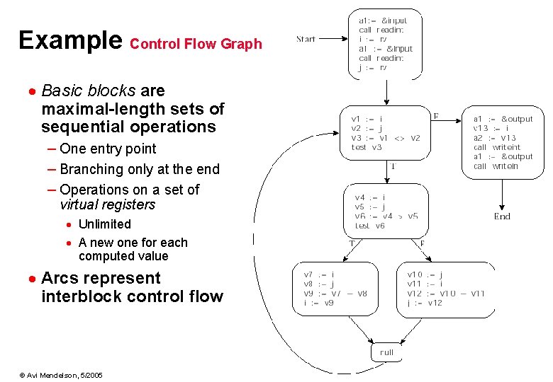
Example Control Flow Graph · Basic blocks are maximal-length sets of sequential operations – One entry point – Branching only at the end – Operations on a set of virtual registers · Unlimited · A new one for each computed value · Arcs represent interblock control flow Lecture 8 – Compiler Optimizations © Avi Mendelson, 5/2005 15

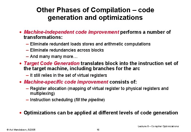
Other Phases of Compilation – code generation and optimizations · Machine-independent code improvement performs a number of transformations: – Eliminate redundant loads stores and arithmetic computations – Eliminate redundancies across blocks – And many more… · Target Code Generation translates block into the instruction set of the target machine, including branches for the arc – It still relies in the set of virtual registers · Machine-specific code improvement consists of: – Register allocation (mapping of virtual register to physical registers and multiplexing) – Instruction scheduling (fill the pipeline) · Optimizations can be applied at different levels of code generation Lecture 8 – Compiler Optimizations © Avi Mendelson, 5/2005 16

General optimization Lecture 8 – Compiler Optimizations © Avi Mendelson, 5/2005 17

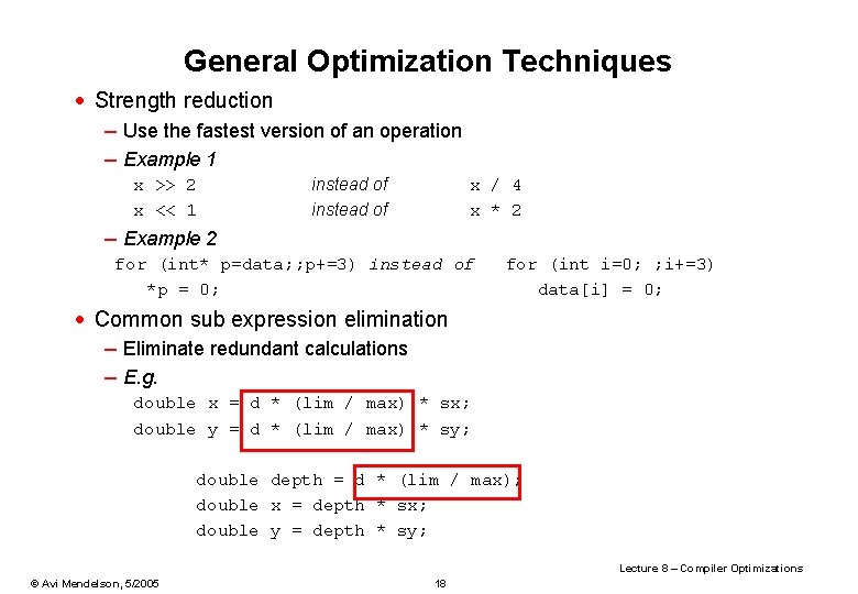
General Optimization Techniques · Strength reduction – Use the fastest version of an operation – Example 1 x >> 2 x << 1 instead of x / 4 x * 2 – Example 2 for (int* p=data; ; p+=3) instead of *p = 0; for (int i=0; ; i+=3) data[i] = 0; · Common sub expression elimination – Eliminate redundant calculations – E. g. double x = d * (lim / max) * sx; double y = d * (lim / max) * sy; double depth = d * (lim / max); double x = depth * sx; double y = depth * sy; Lecture 8 – Compiler Optimizations © Avi Mendelson, 5/2005 18

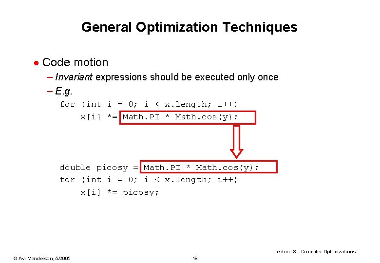
General Optimization Techniques · Code motion – Invariant expressions should be executed only once – E. g. for (int i = 0; i < x. length; i++) x[i] *= Math. PI * Math. cos(y); double picosy = Math. PI * Math. cos(y); for (int i = 0; i < x. length; i++) x[i] *= picosy; Lecture 8 – Compiler Optimizations © Avi Mendelson, 5/2005 19

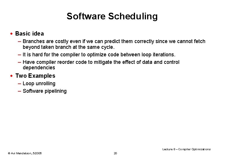
Software Scheduling · Basic idea – Branches are costly even if we can predict them correctly since we cannot fetch beyond taken branch at the same cycle. – It is hard for the compiler to optimize code between loop iterations. – Have compiler reorder code to mitigate the effect of data and control dependencies · Two Examples – Loop unrolling – Software pipelining Lecture 8 – Compiler Optimizations © Avi Mendelson, 5/2005 20

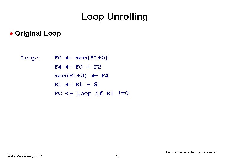
Loop Unrolling · Original Loop: F 0 mem(R 1+0) F 4 F 0 + F 2 mem(R 1+0) F 4 R 1 - 8 PC <- Loop if R 1 !=0 Lecture 8 – Compiler Optimizations © Avi Mendelson, 5/2005 21

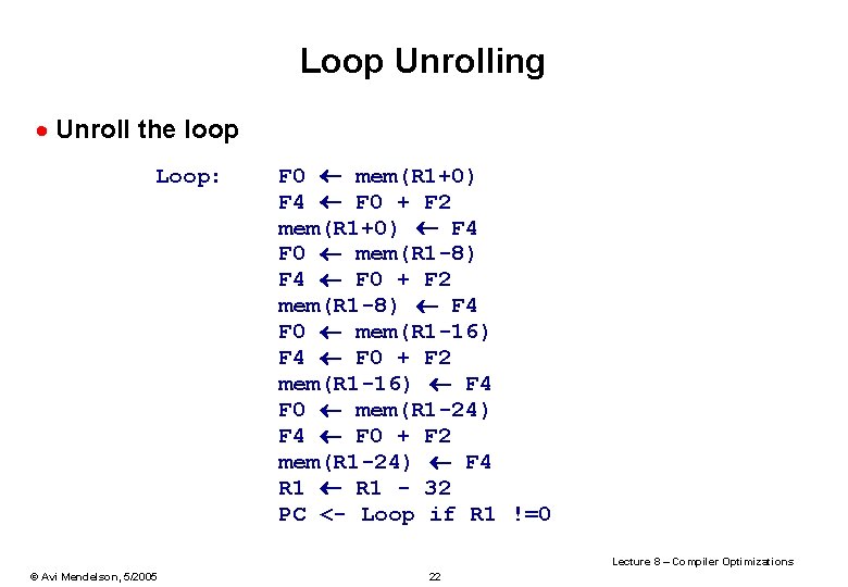
Loop Unrolling · Unroll the loop Loop: F 0 mem(R 1+0) F 4 F 0 + F 2 mem(R 1+0) F 4 F 0 mem(R 1 -8) F 4 F 0 + F 2 mem(R 1 -8) F 4 F 0 mem(R 1 -16) F 4 F 0 + F 2 mem(R 1 -16) F 4 F 0 mem(R 1 -24) F 4 F 0 + F 2 mem(R 1 -24) F 4 R 1 - 32 PC <- Loop if R 1 !=0 Lecture 8 – Compiler Optimizations © Avi Mendelson, 5/2005 22

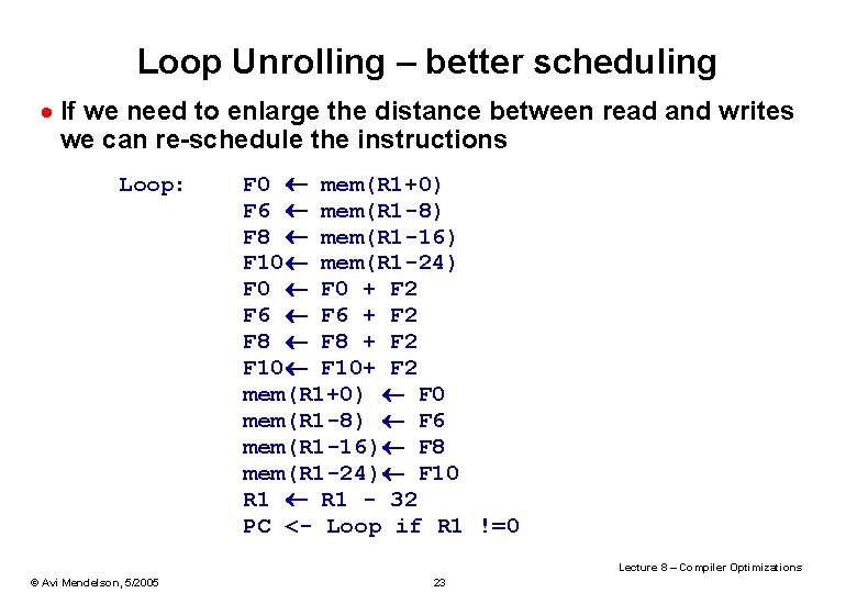
Loop Unrolling – better scheduling · If we need to enlarge the distance between read and writes we can re-schedule the instructions Loop: F 0 mem(R 1+0) F 6 mem(R 1 -8) F 8 mem(R 1 -16) F 10 mem(R 1 -24) F 0 + F 2 F 6 + F 2 F 8 + F 2 F 10+ F 2 mem(R 1+0) F 0 mem(R 1 -8) F 6 mem(R 1 -16) F 8 mem(R 1 -24) F 10 R 1 - 32 PC <- Loop if R 1 !=0 Lecture 8 – Compiler Optimizations © Avi Mendelson, 5/2005 23

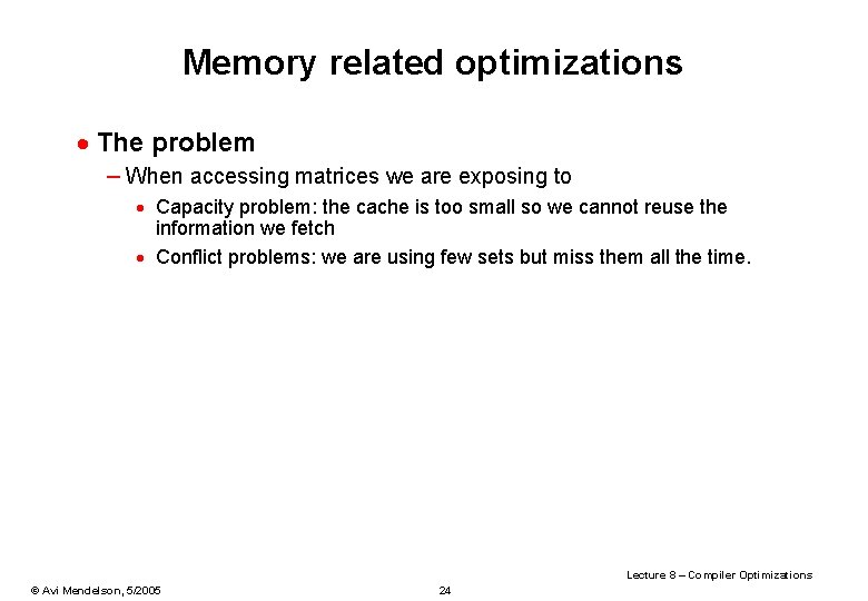
Memory related optimizations · The problem – When accessing matrices we are exposing to · Capacity problem: the cache is too small so we cannot reuse the information we fetch · Conflict problems: we are using few sets but miss them all the time. Lecture 8 – Compiler Optimizations © Avi Mendelson, 5/2005 24

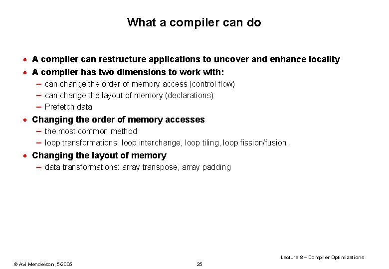
What a compiler can do · A compiler can restructure applications to uncover and enhance locality · A compiler has two dimensions to work with: – can change the order of memory access (control flow) – can change the layout of memory (declarations) – Prefetch data · Changing the order of memory accesses – the most common method – loop transformations: loop interchange, loop tiling, loop fission/fusion, · Changing the layout of memory – data transformations: array transpose, array padding Lecture 8 – Compiler Optimizations © Avi Mendelson, 5/2005 25

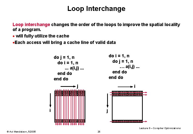
Loop Interchange Loop interchanges the order of the loops to improve the spatial locality of a program. · will fully utilize the cache ·Each access will bring a cache line of valid data do i = 1, n do j = 1, n … a(i, j). . . end do do j = 1, n do i = 1, n. . . a(i, j). . . end do j i i j Lecture 8 – Compiler Optimizations © Avi Mendelson, 5/2005 26

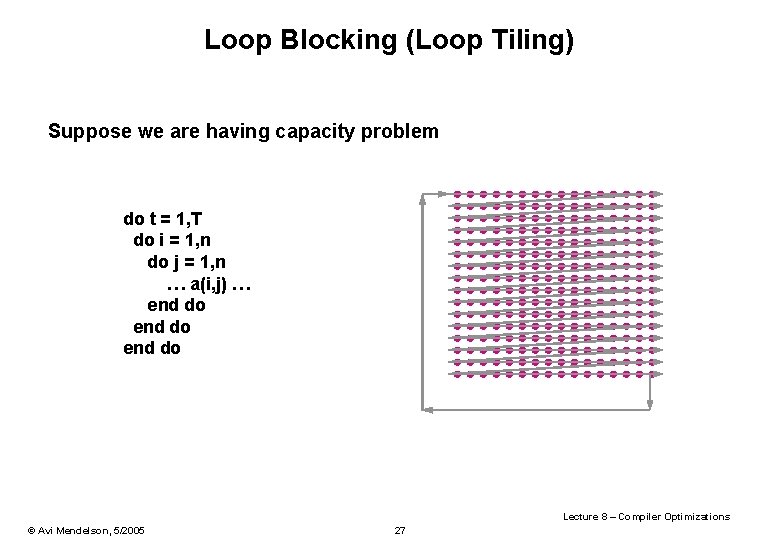
Loop Blocking (Loop Tiling) Suppose we are having capacity problem do t = 1, T do i = 1, n do j = 1, n … a(i, j) … end do Lecture 8 – Compiler Optimizations © Avi Mendelson, 5/2005 27

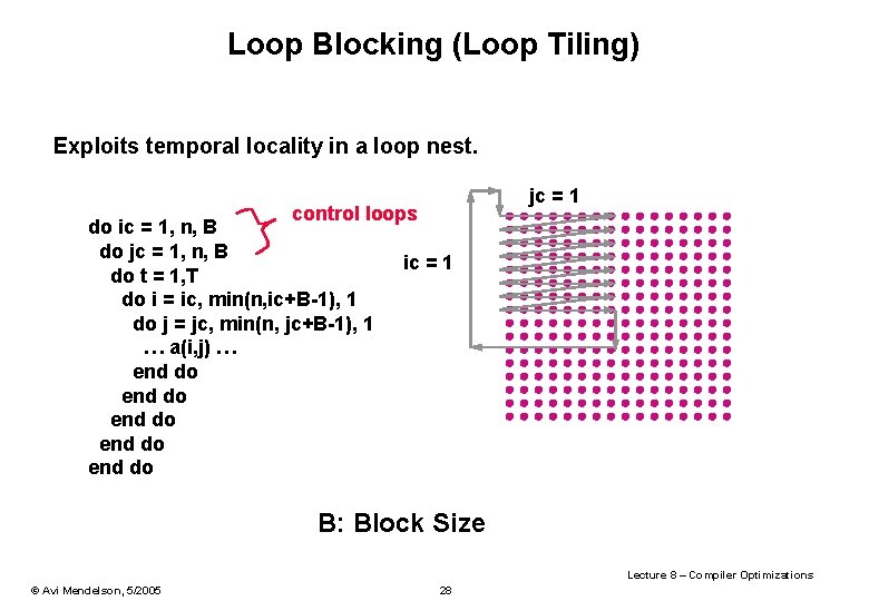
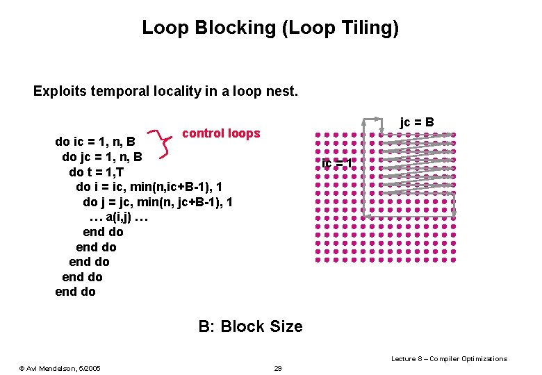
Loop Blocking (Loop Tiling) Exploits temporal locality in a loop nest. control loops do ic = 1, n, B do jc = 1, n, B ic = 1 do t = 1, T do i = ic, min(n, ic+B-1), 1 do j = jc, min(n, jc+B-1), 1 … a(i, j) … end do end do jc = 1 B: Block Size Lecture 8 – Compiler Optimizations © Avi Mendelson, 5/2005 28

Loop Blocking (Loop Tiling) Exploits temporal locality in a loop nest. jc = B control loops do ic = 1, n, B do jc = 1, n, B do t = 1, T do i = ic, min(n, ic+B-1), 1 do j = jc, min(n, jc+B-1), 1 … a(i, j) … end do end do ic = 1 B: Block Size Lecture 8 – Compiler Optimizations © Avi Mendelson, 5/2005 29

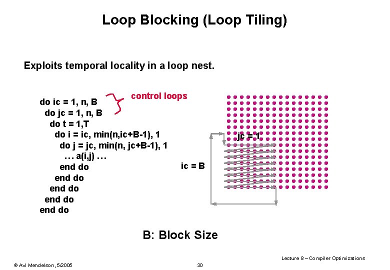
Loop Blocking (Loop Tiling) Exploits temporal locality in a loop nest. control loops do ic = 1, n, B do jc = 1, n, B do t = 1, T do i = ic, min(n, ic+B-1), 1 do j = jc, min(n, jc+B-1), 1 … a(i, j) … ic = B end do end do jc = 1 B: Block Size Lecture 8 – Compiler Optimizations © Avi Mendelson, 5/2005 30

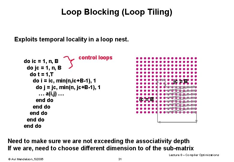
Loop Blocking (Loop Tiling) Exploits temporal locality in a loop nest. control loops do ic = 1, n, B do jc = 1, n, B do t = 1, T do i = ic, min(n, ic+B-1), 1 do j = jc, min(n, jc+B-1), 1 … a(i, j) … end do end do jc = B ic = B Need to make sure we are not exceeding the associativity depth If we are, need to choose different dimension to of the sub-matrix Lecture 8 – Compiler Optimizations © Avi Mendelson, 5/2005 31

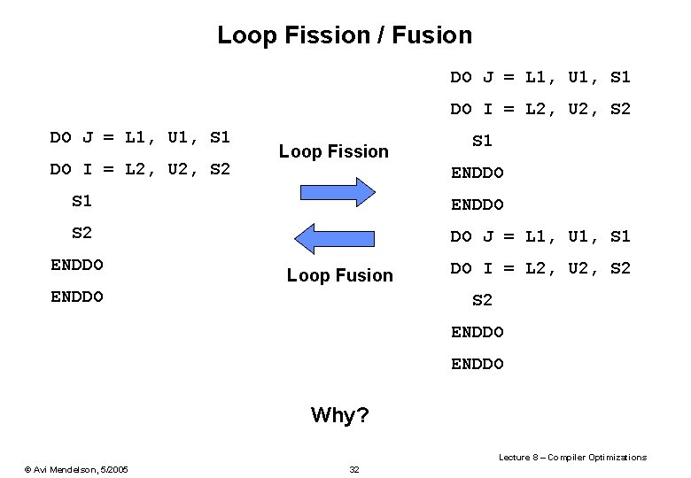
Loop Fission / Fusion DO J = L 1, U 1, S 1 DO I = L 2, U 2, S 2 Loop Fission S 1 ENDDO S 2 DO J = L 1, U 1, S 1 ENDDO Loop Fusion ENDDO DO I = L 2, U 2, S 2 ENDDO Why? Lecture 8 – Compiler Optimizations © Avi Mendelson, 5/2005 32

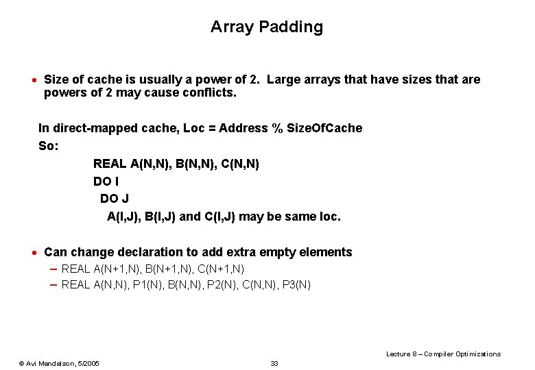
Array Padding · Size of cache is usually a power of 2. Large arrays that have sizes that are powers of 2 may cause conflicts. In direct-mapped cache, Loc = Address % Size. Of. Cache So: REAL A(N, N), B(N, N), C(N, N) DO I DO J A(I, J), B(I, J) and C(I, J) may be same loc. · Can change declaration to add extra empty elements – REAL A(N+1, N), B(N+1, N), C(N+1, N) – REAL A(N, N), P 1(N), B(N, N), P 2(N), C(N, N), P 3(N) Lecture 8 – Compiler Optimizations © Avi Mendelson, 5/2005 33

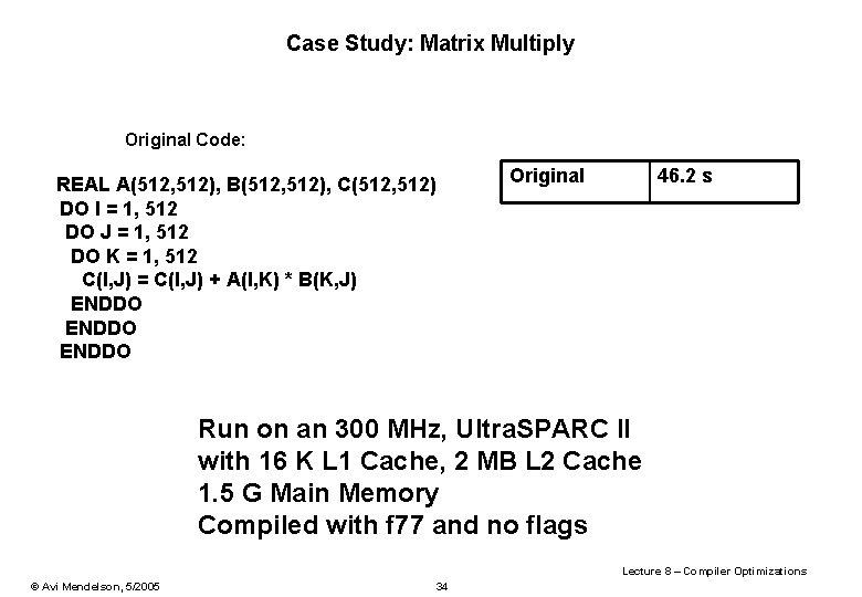
Case Study: Matrix Multiply Original Code: REAL A(512, 512), B(512, 512), C(512, 512) DO I = 1, 512 DO J = 1, 512 DO K = 1, 512 C(I, J) = C(I, J) + A(I, K) * B(K, J) ENDDO Original 46. 2 s Run on an 300 MHz, Ultra. SPARC II with 16 K L 1 Cache, 2 MB L 2 Cache 1. 5 G Main Memory Compiled with f 77 and no flags Lecture 8 – Compiler Optimizations © Avi Mendelson, 5/2005 34

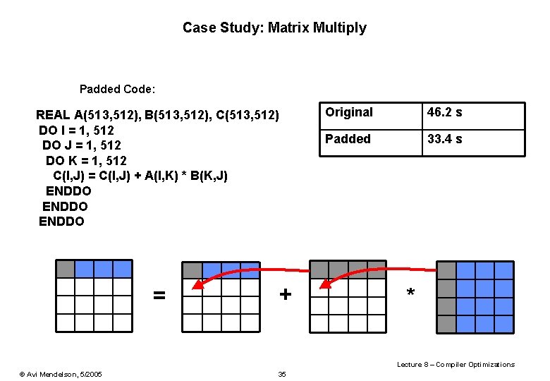
Case Study: Matrix Multiply Padded Code: REAL A(513, 512), B(513, 512), C(513, 512) DO I = 1, 512 DO J = 1, 512 DO K = 1, 512 C(I, J) = C(I, J) + A(I, K) * B(K, J) ENDDO = + Original 46. 2 s Padded 33. 4 s * Lecture 8 – Compiler Optimizations © Avi Mendelson, 5/2005 35

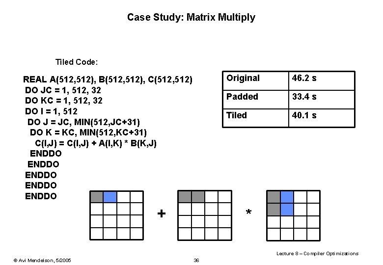
Case Study: Matrix Multiply Tiled Code: REAL A(512, 512), B(512, 512), C(512, 512) DO JC = 1, 512, 32 DO KC = 1, 512, 32 DO I = 1, 512 DO J = JC, MIN(512, JC+31) DO K = KC, MIN(512, KC+31) C(I, J) = C(I, J) + A(I, K) * B(K, J) ENDDO ENDDO + Original 46. 2 s Padded 33. 4 s Tiled 40. 1 s * Lecture 8 – Compiler Optimizations © Avi Mendelson, 5/2005 36

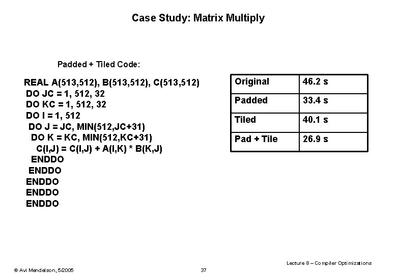
Case Study: Matrix Multiply Padded + Tiled Code: REAL A(513, 512), B(513, 512), C(513, 512) DO JC = 1, 512, 32 DO KC = 1, 512, 32 DO I = 1, 512 DO J = JC, MIN(512, JC+31) DO K = KC, MIN(512, KC+31) C(I, J) = C(I, J) + A(I, K) * B(K, J) ENDDO ENDDO Original 46. 2 s Padded 33. 4 s Tiled 40. 1 s Pad + Tile 26. 9 s Lecture 8 – Compiler Optimizations © Avi Mendelson, 5/2005 37

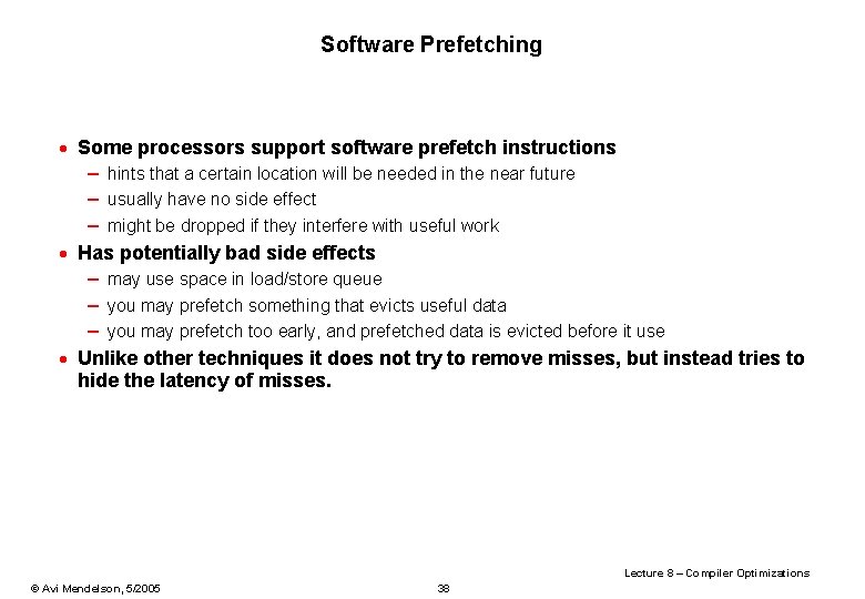
Software Prefetching · Some processors support software prefetch instructions – hints that a certain location will be needed in the near future – usually have no side effect – might be dropped if they interfere with useful work · Has potentially bad side effects – may use space in load/store queue – you may prefetch something that evicts useful data – you may prefetch too early, and prefetched data is evicted before it use · Unlike other techniques it does not try to remove misses, but instead tries to hide the latency of misses. Lecture 8 – Compiler Optimizations © Avi Mendelson, 5/2005 38

Software Prefetch Example: int a; int d[100000][16]; int main() { unsigned i, j, k; for (i=0; i<1000; i++) { for (j=0; j<100000; j++) { prefetch_read(&d[j+5][0]); for (k=0; k<16; k++) { a = a + d[j][k]; } } } for (i=0; i<1000; i++) { for (j=0; j<100000; j++) { for (k=0; k<16; k++) { a = a + d[j][k]; } } } Original 41. 4 s Prefetch 27. 5 s . inline prefetch_read, 1 prefetch [%o 0+0], 0. end Lecture 8 – Compiler Optimizations © Avi Mendelson, 5/2005 39

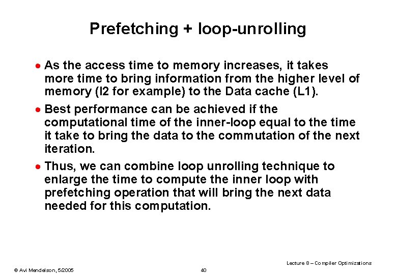
Prefetching + loop-unrolling · As the access time to memory increases, it takes more time to bring information from the higher level of memory (l 2 for example) to the Data cache (L 1). · Best performance can be achieved if the computational time of the inner-loop equal to the time it take to bring the data to the commutation of the next iteration. · Thus, we can combine loop unrolling technique to enlarge the time to compute the inner loop with prefetching operation that will bring the next data needed for this computation. Lecture 8 – Compiler Optimizations © Avi Mendelson, 5/2005 40

Backup Lecture 8 – Compiler Optimizations © Avi Mendelson, 5/2005 41

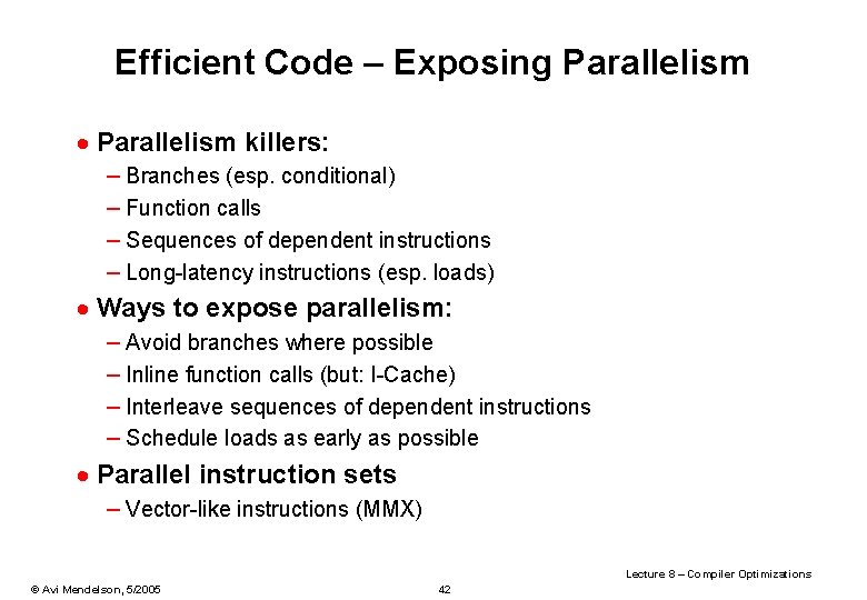
Efficient Code – Exposing Parallelism · Parallelism killers: – Branches (esp. conditional) – Function calls – Sequences of dependent instructions – Long-latency instructions (esp. loads) · Ways to expose parallelism: – Avoid branches where possible – Inline function calls (but: I-Cache) – Interleave sequences of dependent instructions – Schedule loads as early as possible · Parallel instruction sets – Vector-like instructions (MMX) Lecture 8 – Compiler Optimizations © Avi Mendelson, 5/2005 42

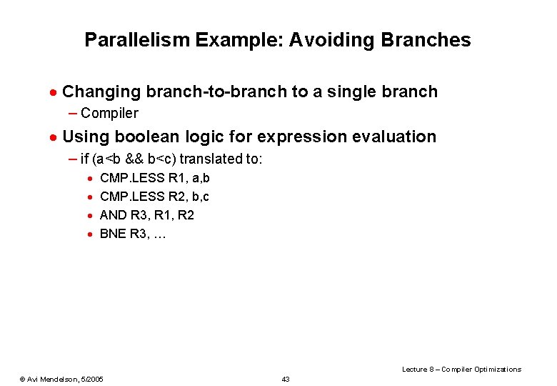
Parallelism Example: Avoiding Branches · Changing branch-to-branch to a single branch – Compiler · Using boolean logic for expression evaluation – if (a<b && b<c) translated to: · · CMP. LESS R 1, a, b CMP. LESS R 2, b, c AND R 3, R 1, R 2 BNE R 3, … Lecture 8 – Compiler Optimizations © Avi Mendelson, 5/2005 43

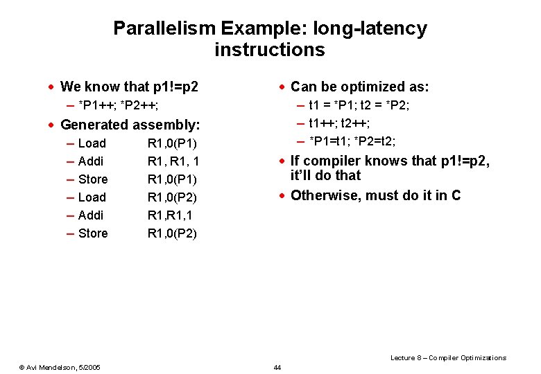
Parallelism Example: long-latency instructions · We know that p 1!=p 2 – *P 1++; *P 2++; · Generated assembly: – Load R 1, 0(P 1) – Addi R 1, 1 – Store R 1, 0(P 1) – Load R 1, 0(P 2) – Addi R 1, 1 – Store R 1, 0(P 2) · Can be optimized as: – t 1 = *P 1; t 2 = *P 2; – t 1++; t 2++; – *P 1=t 1; *P 2=t 2; · If compiler knows that p 1!=p 2, it’ll do that · Otherwise, must do it in C Lecture 8 – Compiler Optimizations © Avi Mendelson, 5/2005 44

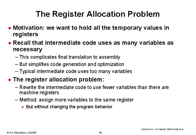
The Register Allocation Problem · Motivation: we want to hold all the temporary values in registers · Recall that intermediate code uses as many variables as necessary – This complicates final translation to assembly – But simplifies code generation and optimization – Typical intermediate code uses too many variables · The register allocation problem: – Rewrite the intermediate code to use fewer variables than there are machine registers – Method: assign more variables to the same register · But without changing the program behavior Lecture 8 – Compiler Optimizations © Avi Mendelson, 5/2005 45

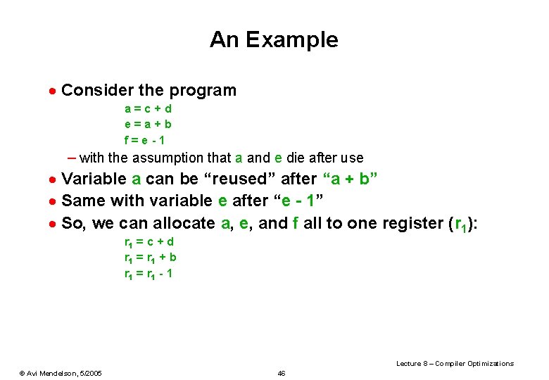
An Example · Consider the program a=c+d e=a+b f=e-1 – with the assumption that a and e die after use · Variable a can be “reused” after “a + b” · Same with variable e after “e - 1” · So, we can allocate a, e, and f all to one register (r 1): r 1 = c + d r 1 = r 1 + b r 1 = r 1 - 1 Lecture 8 – Compiler Optimizations © Avi Mendelson, 5/2005 46

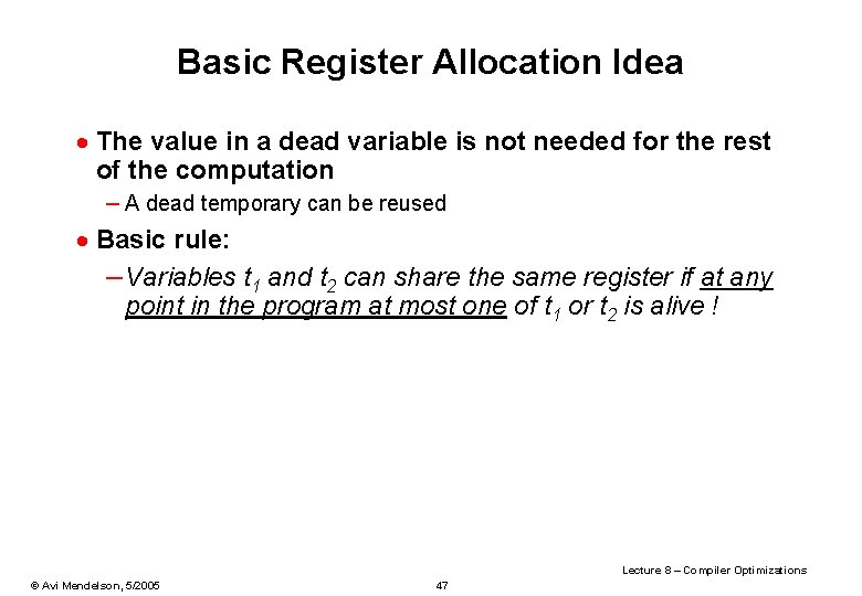
Basic Register Allocation Idea · The value in a dead variable is not needed for the rest of the computation – A dead temporary can be reused · Basic rule: – Variables t 1 and t 2 can share the same register if at any point in the program at most one of t 1 or t 2 is alive ! Lecture 8 – Compiler Optimizations © Avi Mendelson, 5/2005 47

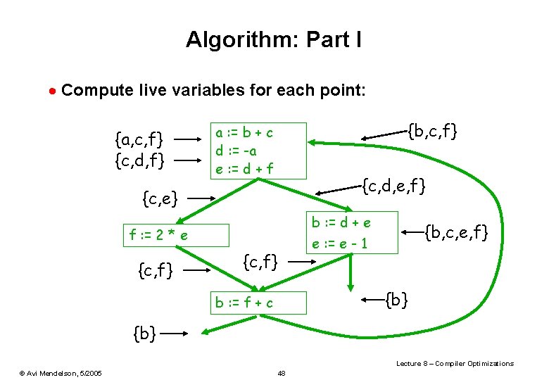
Algorithm: Part I · Compute live variables for each point: {a, c, f} {c, d, f} {b, c, f} a : = b + c d : = -a e : = d + f {c, d, e, f} {c, e} b : = d + e f : = 2 * e {c, f} {b, c, e, f} e : = e - 1 {c, f} {b} b : = f + c {b} Lecture 8 – Compiler Optimizations © Avi Mendelson, 5/2005 48

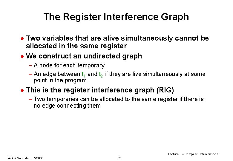
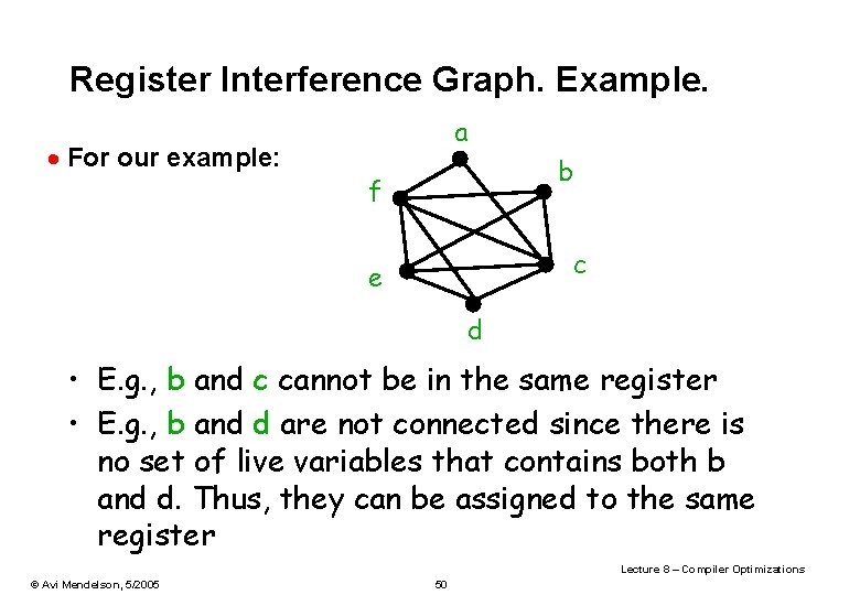
The Register Interference Graph · Two variables that are alive simultaneously cannot be allocated in the same register · We construct an undirected graph – A node for each temporary – An edge between t 1 and t 2 if they are live simultaneously at some point in the program · This is the register interference graph (RIG) – Two temporaries can be allocated to the same register if there is no edge connecting them Lecture 8 – Compiler Optimizations © Avi Mendelson, 5/2005 49

Register Interference Graph. Example. · For our example: a b f c e d • E. g. , b and c cannot be in the same register • E. g. , b and d are not connected since there is no set of live variables that contains both b and d. Thus, they can be assigned to the same register Lecture 8 – Compiler Optimizations © Avi Mendelson, 5/2005 50

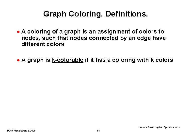
Graph Coloring. Definitions. · A coloring of a graph is an assignment of colors to nodes, such that nodes connected by an edge have different colors · A graph is k-colorable if it has a coloring with k colors Lecture 8 – Compiler Optimizations © Avi Mendelson, 5/2005 51

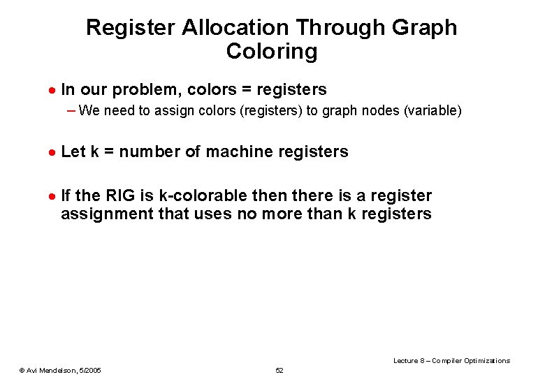
Register Allocation Through Graph Coloring · In our problem, colors = registers – We need to assign colors (registers) to graph nodes (variable) · Let k = number of machine registers · If the RIG is k-colorable then there is a register assignment that uses no more than k registers Lecture 8 – Compiler Optimizations © Avi Mendelson, 5/2005 52

Problems with Graph coloring approach · This is a well known NP-complete problem – We need to use heuristics · What’s happen if we cannot color the graph with K colors (assuming K is the number of the general purpose architectural registers – We need to use “Register Spilling” Lecture 8 – Compiler Optimizations © Avi Mendelson, 5/2005 53

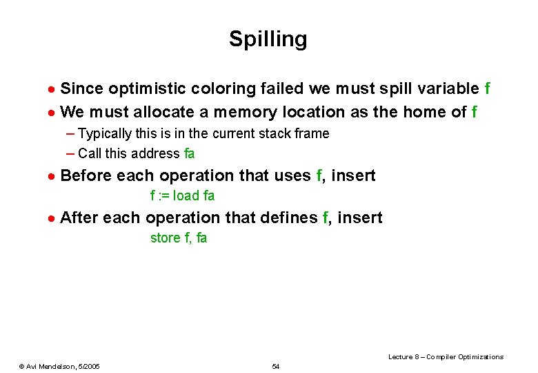
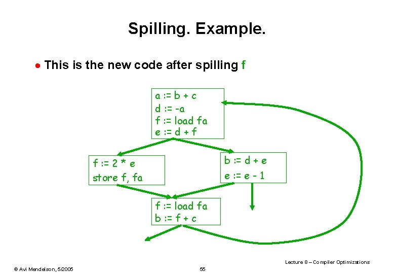
Spilling · Since optimistic coloring failed we must spill variable f · We must allocate a memory location as the home of f – Typically this is in the current stack frame – Call this address fa · Before each operation that uses f, insert f : = load fa · After each operation that defines f, insert store f, fa Lecture 8 – Compiler Optimizations © Avi Mendelson, 5/2005 54

Spilling. Example. · This is the new code after spilling f a : = b + c d : = -a f : = load fa e : = d + f b : = d + e f : = 2 * e store f, fa e : = e - 1 f : = load fa b : = f + c Lecture 8 – Compiler Optimizations © Avi Mendelson, 5/2005 55

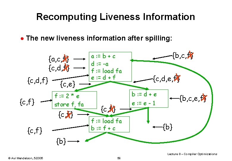
Recomputing Liveness Information · The new liveness information after spilling: {a, c, f} {c, d, f} {c, e} f : = 2 * e store f, fa {c, f} a : = b + c d : = -a f : = load fa e : = d + f {b, c, f} {c, d, e, f} b : = d + e {b, c, e, f} e : = e - 1 {c, f} f : = load fa b : = f + c {b} Lecture 8 – Compiler Optimizations © Avi Mendelson, 5/2005 56

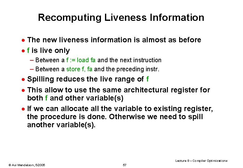
Recomputing Liveness Information · The new liveness information is almost as before · f is live only – Between a f : = load fa and the next instruction – Between a store f, fa and the preceding instr. · Spilling reduces the live range of f · This allow to use the same architectural register for both f and other variable(s) · If we can allocate all the variable to existing register, the procedure is done. Otherwise we need to spill another variable(s). Lecture 8 – Compiler Optimizations © Avi Mendelson, 5/2005 57

Software Pipelining [Charlesworth 1981] q Overlap multiple loop iterations in single loop body • Requires Start up Code Main Loop Body Finish up code q Example sum = 0. 0; for (i=1; i<=N; i++) { v 1=load v 2=load v 3=mult sum=add ; sum = sum+a[i]*b[i] a[i] b[i] v 1, v 2 sum, v 3 } Lecture 8 – Compiler Optimizations © Avi Mendelson, 5/2005 58

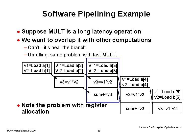
Software Pipelining Example · Suppose MULT is a long latency operation · We want to overlap it with other computations – Can’t - it’s near the branch. – Unrolling: same problem with last MULT. v 1=Load a[1] v 2=Load b[1] V’ 1=Load a[2] V’ 2=Load b[2] V’’ 1=Load a[3] V’’ 2=Load b[3] v 3=v 1*v 2 v 1=Load a[4] v 2=Load b[4] sum+=v 3 v 3=v 1*v 2 v 1=Load a[5] v 2=Load b[5] sum+=v 3 v 3=v 1*v 2 · Note the problem with register allocation Lecture 8 – Compiler Optimizations © Avi Mendelson, 5/2005 59

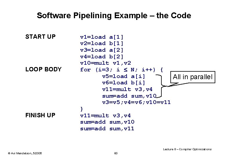
Software Pipelining Example – the Code START UP LOOP BODY FINISH UP v 1=load a[1] v 2=load b[1] v 3=load a[2] v 4=load b[2] v 10=mult v 1, v 2 for (i=3; i N; i++) { v 5=load a[i] All in parallel v 6=load b[i] v 11=mult v 3, v 4 sum=add sum, v 10 v 3=v 5; v 4=v 6; v 10=v 11 } v 11=mult v 3, v 4 sum=add sum, v 10 sum=add sum, v 11 Lecture 8 – Compiler Optimizations © Avi Mendelson, 5/2005 60