Lecture 10 Code Optimization CS 5363 Programming Languages

Lecture 10 Code Optimization CS 5363 Programming Languages and Compilers Xiaoyin Wang

Compiler Code Optimizations • Introduction – Optimized code • Executes faster • efficient memory usage • yielding better performance. – Compilers can be designed to provide code optimization. – Users should only focus on optimizations not provided by the compiler such as choosing a faster and/or less memory intensive algorithm

Compiler Code Optimizations • A Code optimizer sits between the front end and the code generator. – Works with intermediate code. – Perform various analysis on the code – Does transformations to improve the intermediate code.

Code Optimization • Machine Independent Optimizations – Done in the AST level, or 3 -address code level – Do not consider the machine architecture • Machine Dependent Optimizations – Typically done when generating machine code – Need to consider instructions set, register availability

Code Analysis Techniques • A lot of MI/MD optimization needs analysis to be implemented – Common expression reduction – Register allocation – Constant propagation – Dead assignment elimination –…

Code Analysis Techniques • Data flow analysis, Points-to analysis, Call -graph analysis, … • Data flow analysis – Used most widely in code optimization – Basis of other analysis

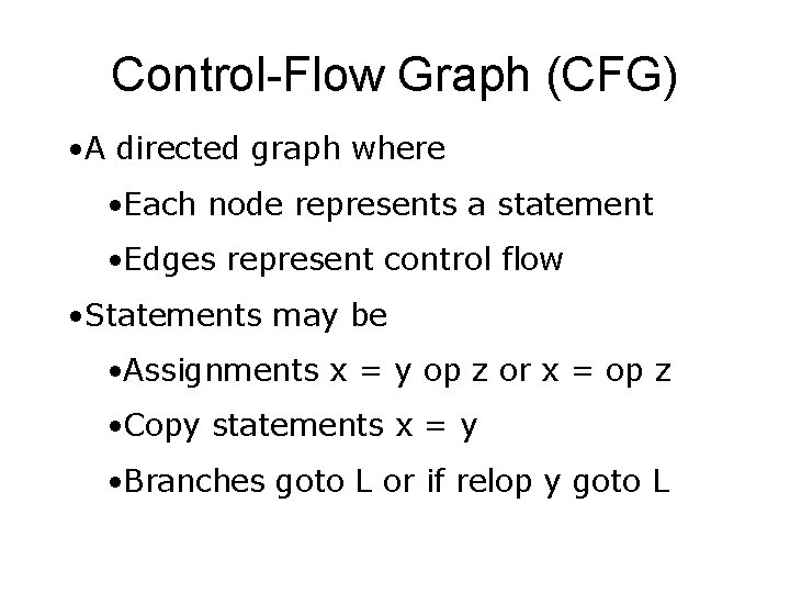
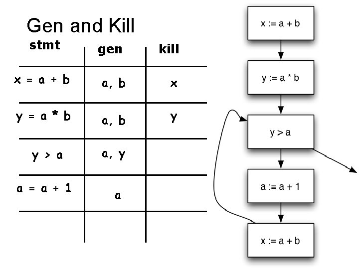
Control-Flow Graph (CFG) • A directed graph where • Each node represents a statement • Edges represent control flow • Statements may be • Assignments x = y op z or x = op z • Copy statements x = y • Branches goto L or if relop y goto L

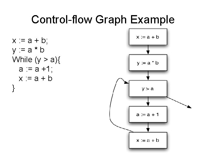
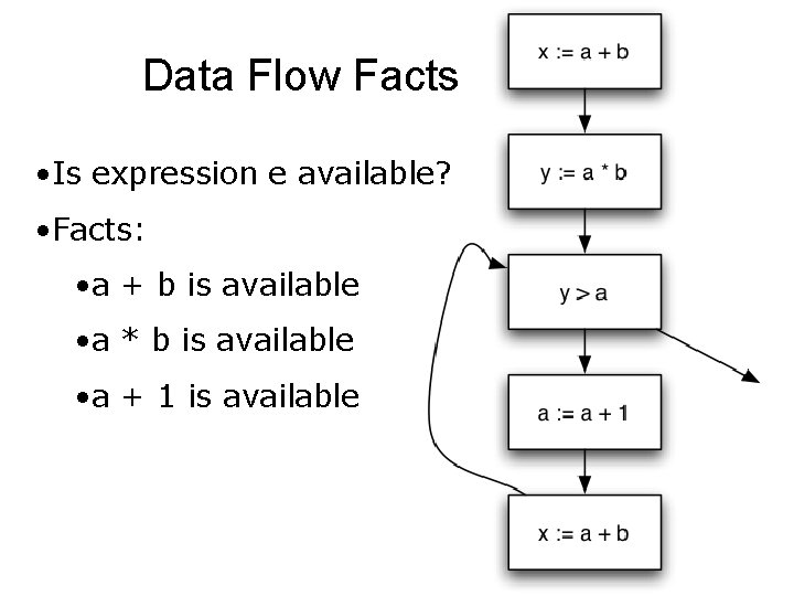
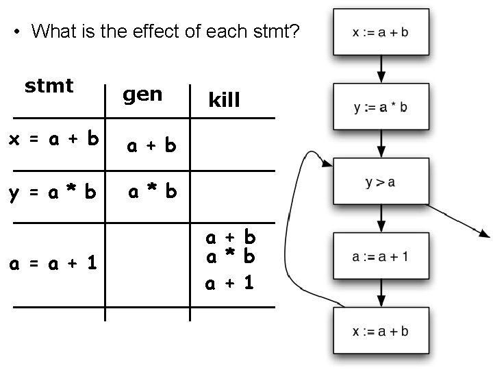
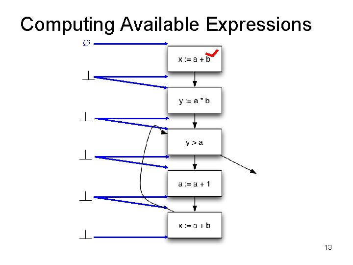
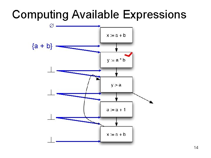
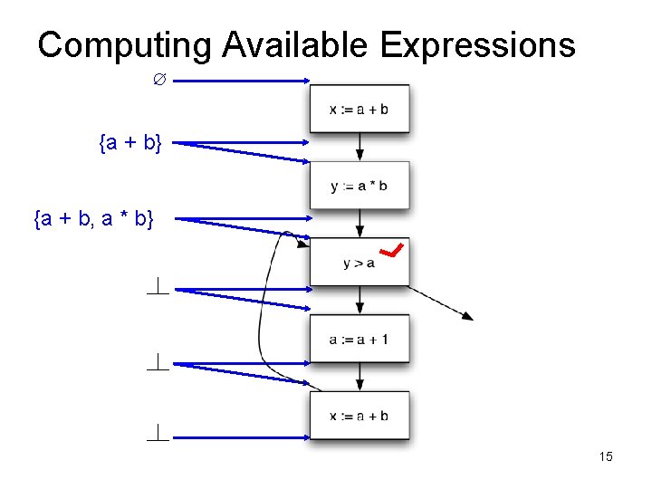
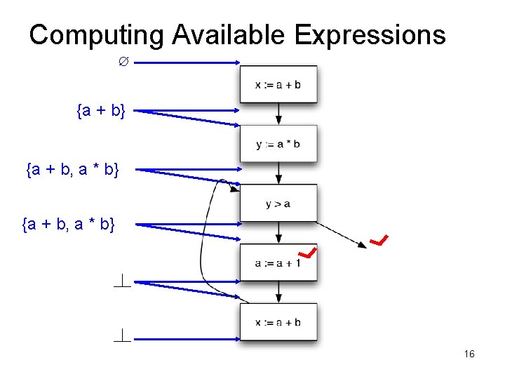
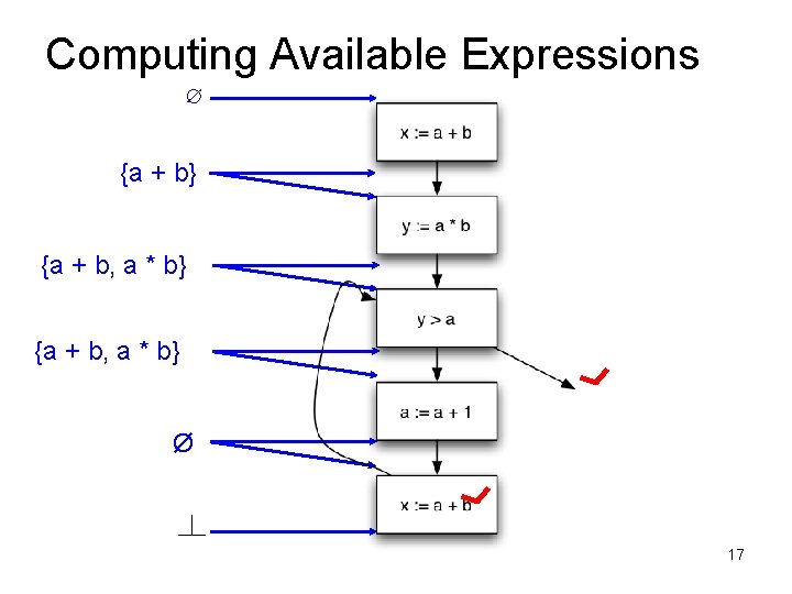
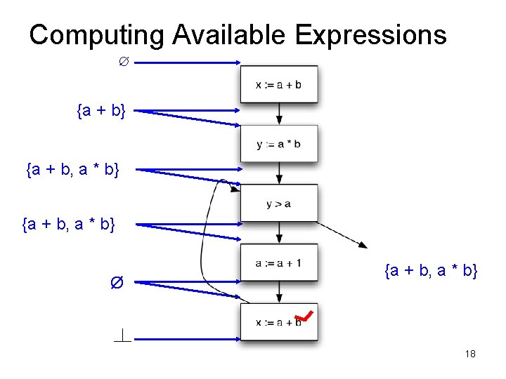
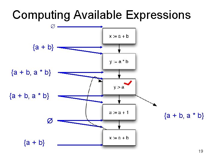
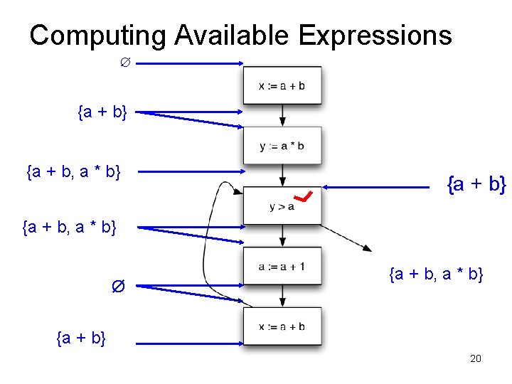
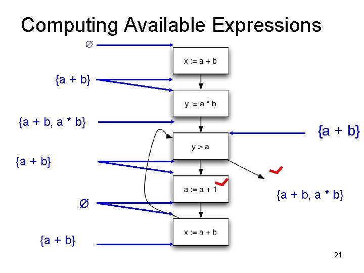
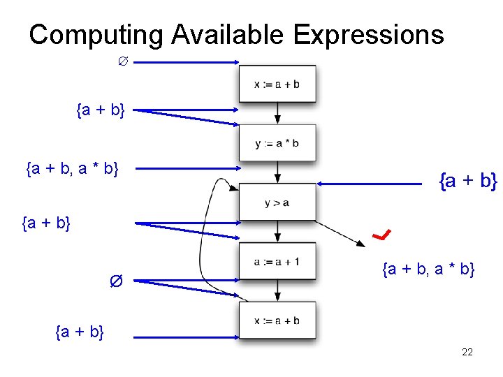
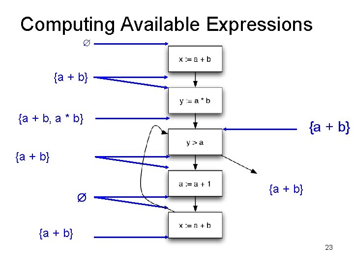
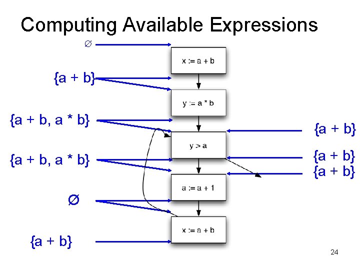
Control-flow Graph Example x : = a + b; y : = a * b While (y > a){ a : = a +1; x : = a + b }

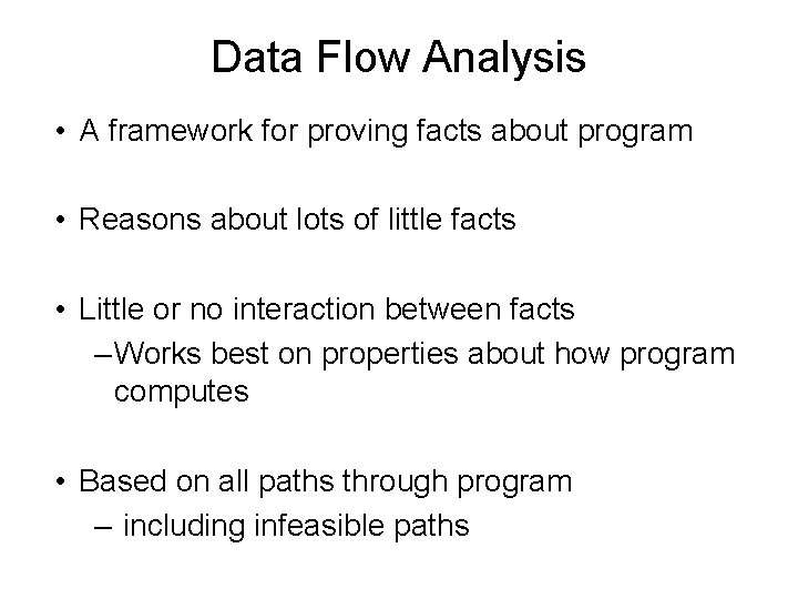
Data Flow Analysis • A framework for proving facts about program • Reasons about lots of little facts • Little or no interaction between facts – Works best on properties about how program computes • Based on all paths through program – including infeasible paths

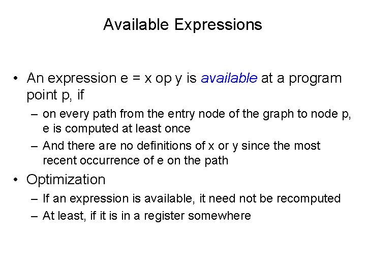
Available Expressions • An expression e = x op y is available at a program point p, if – on every path from the entry node of the graph to node p, e is computed at least once – And there are no definitions of x or y since the most recent occurrence of e on the path • Optimization – If an expression is available, it need not be recomputed – At least, if it is in a register somewhere

Data Flow Facts • Is expression e available? • Facts: • a + b is available • a * b is available • a + 1 is available

• What is the effect of each stmt? stmt gen x = a + b y = a * b a = a + 1 kill a + b a * b a + 1

Computing Available Expressions ∅ 13

Computing Available Expressions ∅ {a + b} 14

Computing Available Expressions ∅ {a + b} {a + b, a * b} 15

Computing Available Expressions ∅ {a + b} {a + b, a * b} 16

Computing Available Expressions ∅ {a + b} {a + b, a * b} Ø 17

Computing Available Expressions ∅ {a + b} {a + b, a * b} Ø {a + b, a * b} 18

Computing Available Expressions ∅ {a + b} {a + b, a * b} Ø {a + b, a * b} {a + b} 19

Computing Available Expressions ∅ {a + b} {a + b, a * b} Ø {a + b, a * b} {a + b} 20

Computing Available Expressions ∅ {a + b} {a + b, a * b} {a + b} Ø {a + b, a * b} {a + b} 21

Computing Available Expressions ∅ {a + b} {a + b, a * b} {a + b} Ø {a + b, a * b} {a + b} 22

Computing Available Expressions ∅ {a + b} {a + b, a * b} {a + b} Ø {a + b} 23

Computing Available Expressions ∅ {a + b} {a + b, a * b} {a + b} Ø {a + b} 24

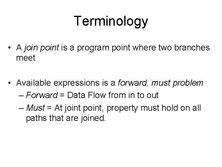
Terminology • A join point is a program point where two branches meet • Available expressions is a forward, must problem – Forward = Data Flow from in to out – Must = At joint point, property must hold on all paths that are joined.

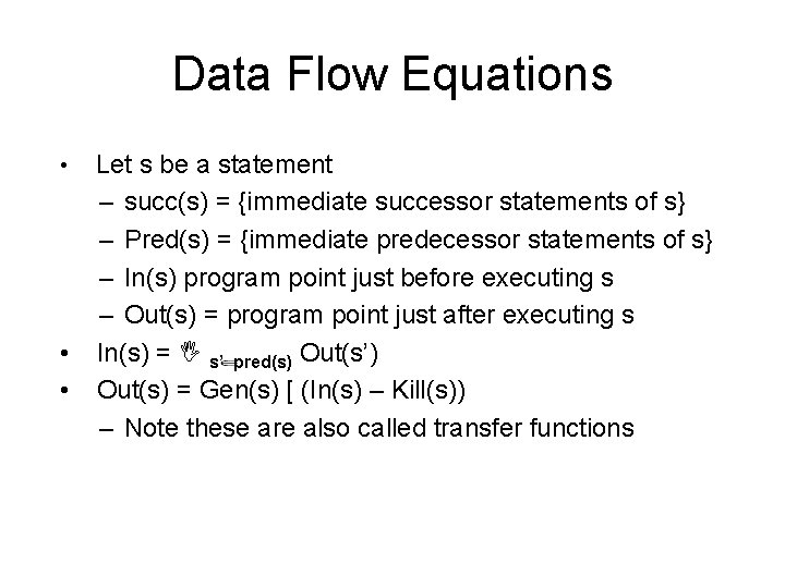
Data Flow Equations Let s be a statement – succ(s) = {immediate successor statements of s} – Pred(s) = {immediate predecessor statements of s} – In(s) program point just before executing s – Out(s) = program point just after executing s • In(s) = I s’ pred(s) Out(s’) • Out(s) = Gen(s) [ (In(s) – Kill(s)) – Note these are also called transfer functions •

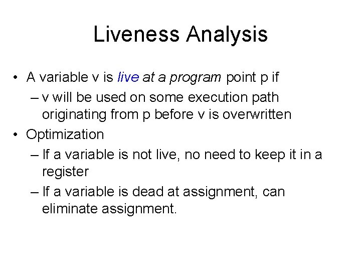
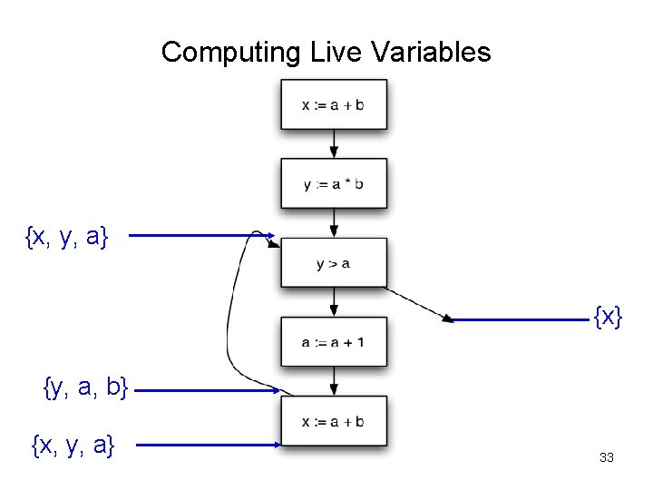
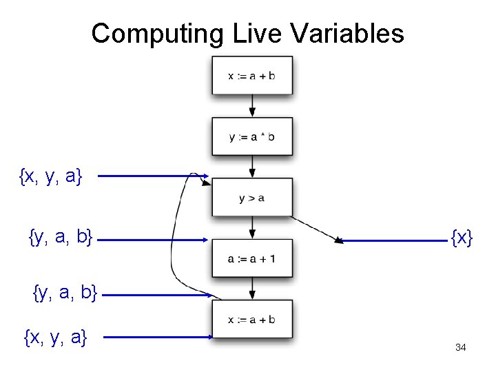
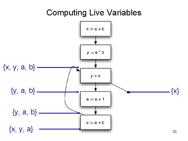
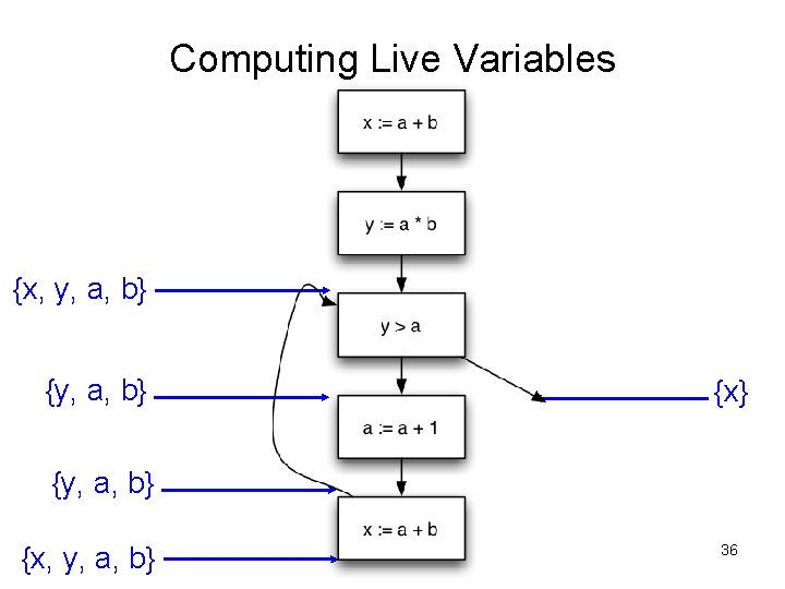
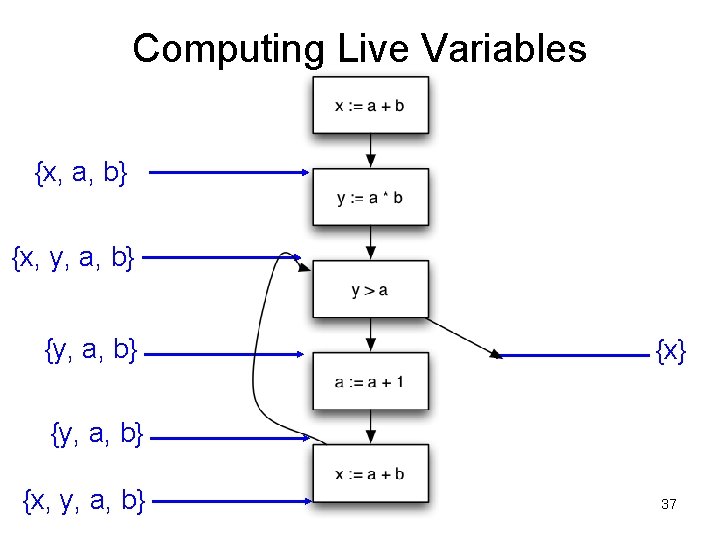
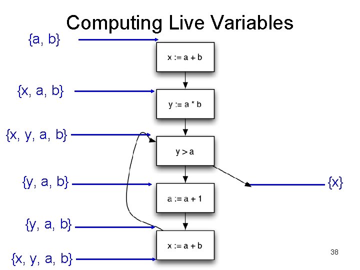
Liveness Analysis • A variable v is live at a program point p if – v will be used on some execution path originating from p before v is overwritten • Optimization – If a variable is not live, no need to keep it in a register – If a variable is dead at assignment, can eliminate assignment.

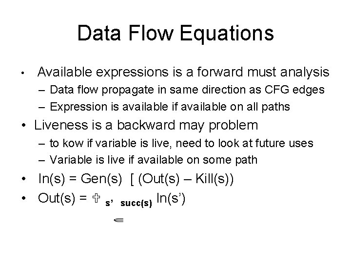
Data Flow Equations • Available expressions is a forward must analysis – Data flow propagate in same direction as CFG edges – Expression is available if available on all paths • Liveness is a backward may problem – to kow if variable is live, need to look at future uses – Variable is live if available on some path • In(s) = Gen(s) [ (Out(s) – Kill(s)) • Out(s) = U s’ succ(s) In(s’)

Gen and Kill stmt gen kill x = a + b a, b x y = a * b a, b y y > a a = a + 1 a, y a

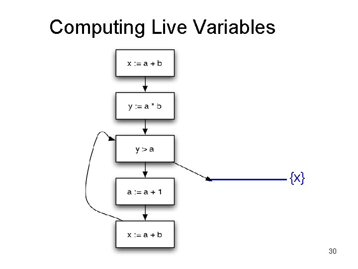
Computing Live Variables {x} 30

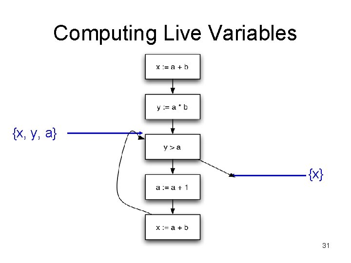
Computing Live Variables {x, y, a} {x} 31

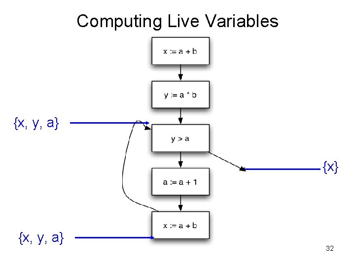
Computing Live Variables {x, y, a} 32

Computing Live Variables {x, y, a} {x} {y, a, b} {x, y, a} 33

Computing Live Variables {x, y, a} {y, a, b} {x, y, a} 34

Computing Live Variables {x, y, a, b} {x} {y, a, b} {x, y, a} 35

Computing Live Variables {x, y, a, b} {x} {y, a, b} {x, y, a, b} 36

Computing Live Variables {x, a, b} {x, y, a, b} {x} {y, a, b} {x, y, a, b} 37

{a, b} Computing Live Variables {x, a, b} {x, y, a, b} {x} {y, a, b} {x, y, a, b} 38

Other Basic Machine Independent Optimizations • Some popular ones: – Inlining small functions – Code hoisting – Dead store elimination – Eliminating common sub-expressions – Loop optimizations: Code motion, Induction variable elimination, and Reduction in strength.

Machine Independent Optimizations • Inlining small functions – Repeatedly inserting the function code instead of calling it, saves the calling overhead and enable further optimizations. – Inlining large functions will make the executable too large.

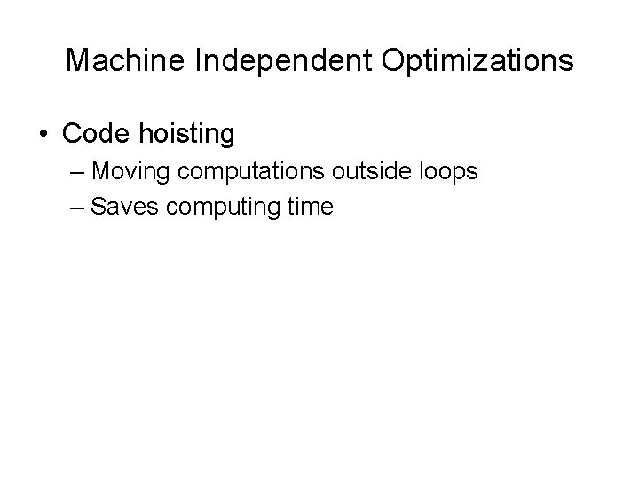
Machine Independent Optimizations • Code hoisting – Moving computations outside loops – Saves computing time

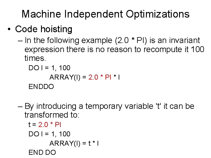
Machine Independent Optimizations • Code hoisting – In the following example (2. 0 * PI) is an invariant expression there is no reason to recompute it 100 times. DO I = 1, 100 ARRAY(I) = 2. 0 * PI * I ENDDO – By introducing a temporary variable 't' it can be transformed to: t = 2. 0 * PI DO I = 1, 100 ARRAY(I) = t * I END DO

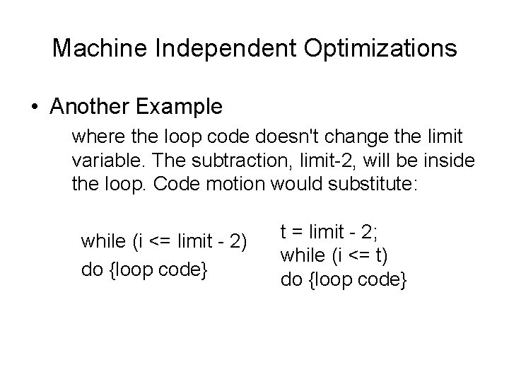
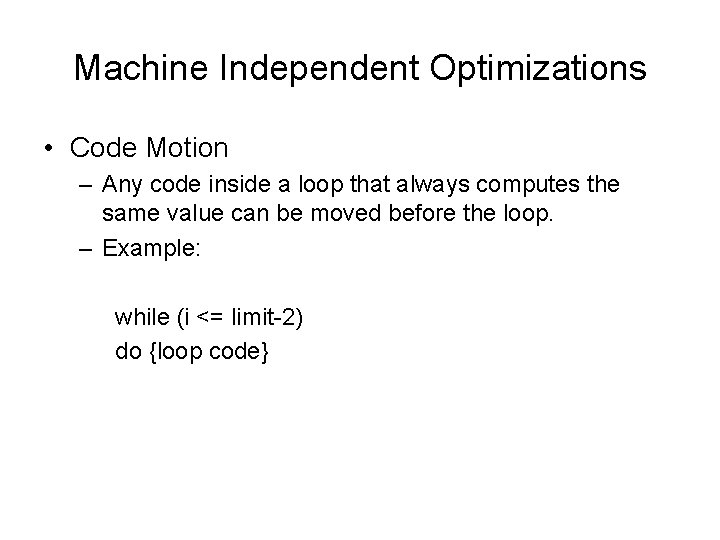
Machine Independent Optimizations • Another Example where the loop code doesn't change the limit variable. The subtraction, limit-2, will be inside the loop. Code motion would substitute: while (i <= limit - 2) do {loop code} t = limit - 2; while (i <= t) do {loop code}

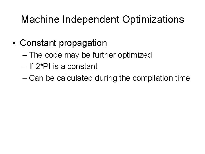
Machine Independent Optimizations • Constant propagation – The code may be further optimized – If 2*PI is a constant – Can be calculated during the compilation time

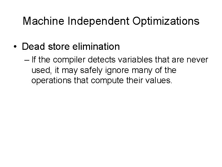
Machine Independent Optimizations • Dead store elimination – If the compiler detects variables that are never used, it may safely ignore many of the operations that compute their values.

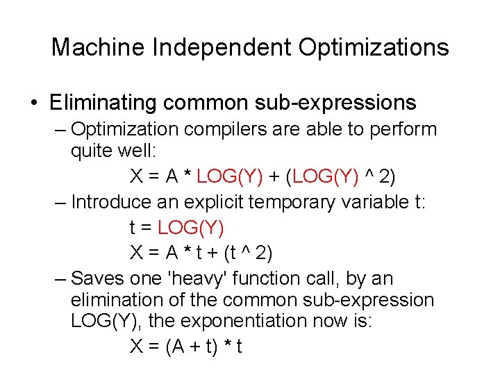
Machine Independent Optimizations • Eliminating common sub-expressions – Optimization compilers are able to perform quite well: X = A * LOG(Y) + (LOG(Y) ^ 2) – Introduce an explicit temporary variable t: t = LOG(Y) X = A * t + (t ^ 2) – Saves one 'heavy' function call, by an elimination of the common sub-expression LOG(Y), the exponentiation now is: X = (A + t) * t

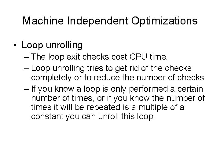
Machine Independent Optimizations • Loop unrolling – The loop exit checks cost CPU time. – Loop unrolling tries to get rid of the checks completely or to reduce the number of checks. – If you know a loop is only performed a certain number of times, or if you know the number of times it will be repeated is a multiple of a constant you can unroll this loop.

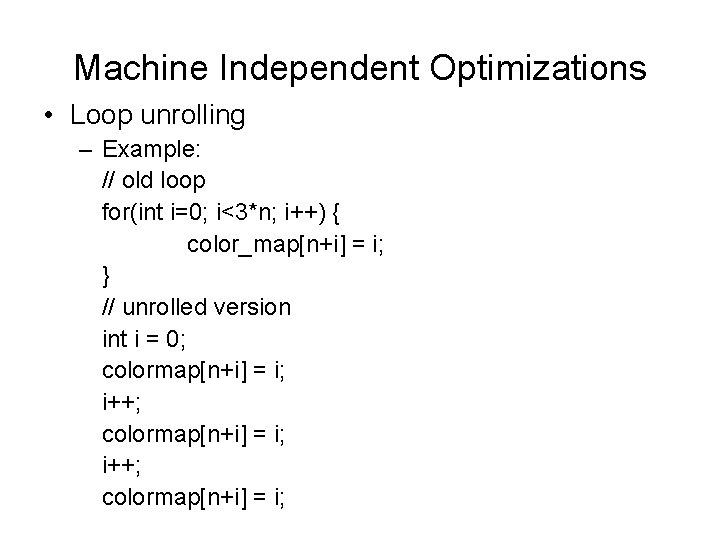
Machine Independent Optimizations • Loop unrolling – Example: // old loop for(int i=0; i<3*n; i++) { color_map[n+i] = i; } // unrolled version int i = 0; colormap[n+i] = i; i++; colormap[n+i] = i;

Machine Independent Optimizations • Code Motion – Any code inside a loop that always computes the same value can be moved before the loop. – Example: while (i <= limit-2) do {loop code}

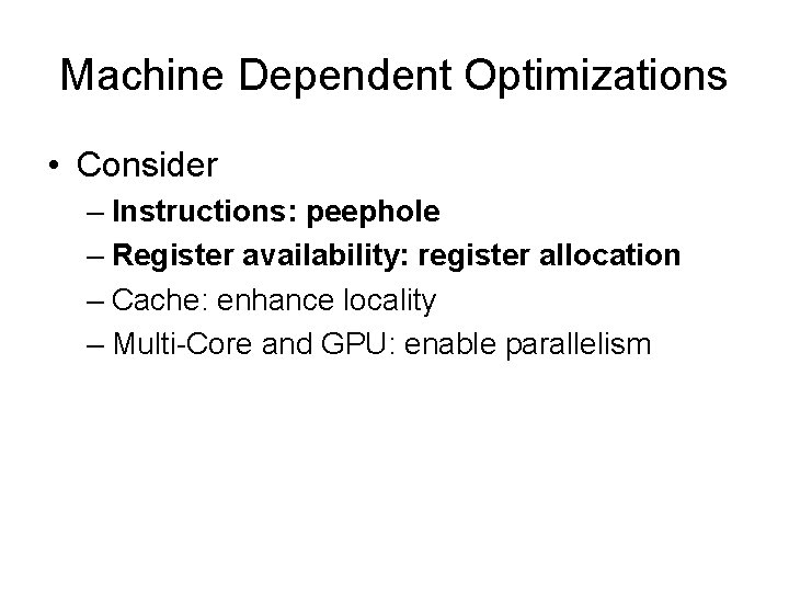
Machine Dependent Optimizations • Consider – Instructions: peephole – Register availability: register allocation – Cache: enhance locality – Multi-Core and GPU: enable parallelism

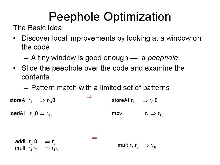
Peephole Optimization The Basic Idea • Discover local improvements by looking at a window on the code – A tiny window is good enough — a peephole • Slide the peephole over the code and examine the contents – Pattern match with a limited set of patterns store. AI r 1 r 0, 8 store. AI r 1 load. AI r 0, 8 r 15 add. I r 2, 0 mult r 4, r 7 r 10 mov r 0, 8 r 15 mult r 4, r 2 r 10

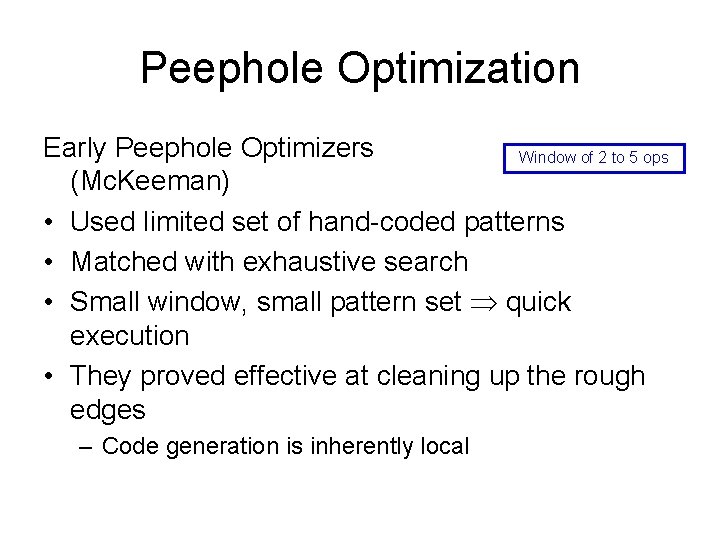
Peephole Optimization Early Peephole Optimizers Window of 2 to 5 ops (Mc. Keeman) • Used limited set of hand-coded patterns • Matched with exhaustive search • Small window, small pattern set quick execution • They proved effective at cleaning up the rough edges – Code generation is inherently local

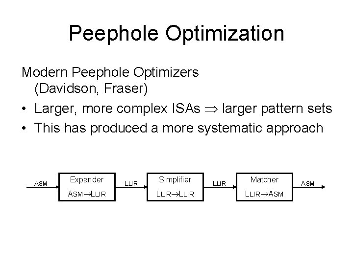
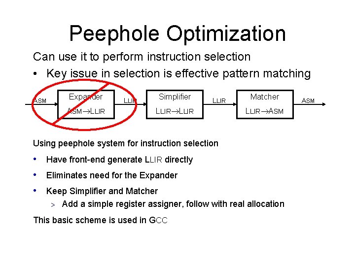
Peephole Optimization Modern Peephole Optimizers (Davidson, Fraser) • Larger, more complex ISAs larger pattern sets • This has produced a more systematic approach ASM Expander ASM LLIR Simplifier LLIR Matcher LLIR ASM

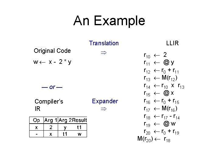
Peephole Optimization Expander • Operation-by-operation expansion into LLIR • Needs no context • Captures full effect of an operation

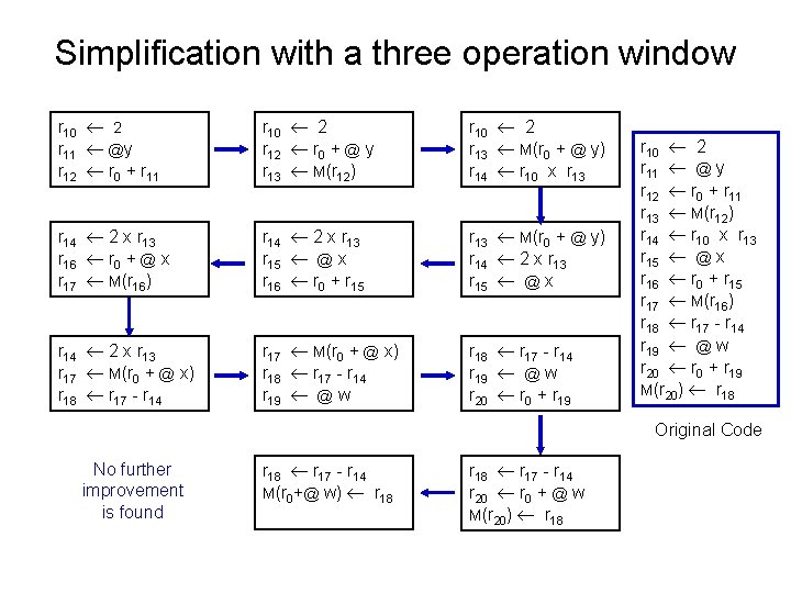
Peephole Optimization Simplifier • Single pass over LLIR, moving the peephole • Forward substitution, algebraic simplification, constant folding, & eliminating useless effects (must know what is dead ) • Eliminate as many LLIR operations as possible

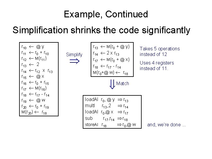
Peephole Optimization Matcher • Starts with reduced LLIR program • Compares LLIR from peephole against pattern library • Selects one or more ASM patterns that “cover” the LLIR – Capture all of its effects – May create new useless effects

Peephole Optimization Can use it to perform instruction selection • Key issue in selection is effective pattern matching Expander ASM LLIR Simplifier LLIR Matcher LLIR ASM Using peephole system for instruction selection • Have front-end generate LLIR directly • Eliminates need for the Expander • Keep Simplifier and Matcher > Add a simple register assigner, follow with real allocation This basic scheme is used in GCC ASM

An Example Translation Original Code w x- 2*y — or — Compiler’s IR Expander LLIR r 10 2 r 11 @ y r 12 r 0 + r 11 r 13 M(r 12) r 14 r 10 x r 13 r 15 @ x r 16 r 0 + r 15 r 17 M(r 16) r 18 r 17 - r 14 r 19 @ w r 20 r 0 + r 19 M(r 20) r 18

Simplification with a three operation window r 10 2 r 11 @y r 12 r 0 + r 11 r 10 2 r 12 r 0 + @ y r 13 M(r 12) r 10 2 r 13 M(r 0 + @ y) r 14 r 10 x r 13 r 14 2 x r 13 r 16 r 0 + @ x r 17 M(r 16) r 14 2 x r 13 r 15 @ x r 16 r 0 + r 15 r 13 M(r 0 + @ y) r 14 2 x r 13 r 15 @ x r 14 2 x r 13 r 17 M(r 0 + @ x) r 18 r 17 - r 14 r 19 @ w r 20 r 0 + r 19 r 10 2 r 11 @ y r 12 r 0 + r 11 r 13 M(r 12) r 14 r 10 x r 13 r 15 @ x r 16 r 0 + r 15 r 17 M(r 16) r 18 r 17 - r 14 r 19 @ w r 20 r 0 + r 19 M(r 20) r 18 Original Code No further improvement is found r 18 r 17 - r 14 M(r 0+@ w) r 18 r 17 - r 14 r 20 r 0 + @ w M(r 20) r 18

Example, Continued Simplification shrinks the code significantly r 10 @ y r 11 r 0 + r 10 r 12 M(r 11) r 13 2 r 14 r 12 x r 13 r 15 @ x r 16 r 0 + r 15 r 17 M(r 16) r 18 r 17 - r 14 r 19 @ w r 20 r 0 + r 19 M(r 20) r 18 Simplify r 13 M(r 0 + @ y) r 14 2 x r 13 r 17 M(r 0 + @ x) r 18 r 17 - r 14 M(r 0+@ w) r 18 Takes 5 operations instead of 12 Uses 4 registers instead of 11. Match load. AI mult. I load. AI sub r 0, @ y r 13, 2 r 0, @ x r 17, r 14 store. AI r 18 r 13 r 14 r 17 r 18 r 0 , @ w and, we’re done. . .