CSE 551 Computational Methods 20182019 Fall Chapter 4

CSE 551 Computational Methods 2018/2019 Fall Chapter 4 Locating Roots of Equations

Outline Bisection Method Newton’s Method Secant method

References • W. Cheney, D Kincaid, Numerical Mathematics and Computing, 6 ed, • Chapter 3

Bisction Method Introduction Bisection Algor, thm and Pseudocode Examples Convergence Analysis False Position (Regula Falsi) Me 4 thod and Modifications

Introduction • Let f be a real- or complex-valued function of a real or complex variable • A number r - real or complex - f (r ) = 0 • a root of that equation or a zero of f • e. g. , f (x) = 6 x 2 − 7 x + 2 • has 1/2 and 2/3 as zeros, verified • by direct substitution or • by writing f in its factored form: f (x) = (2 x − 1)(3 x − 2)

g(x) = cos 3 x − cos 7 x • not only x = 0 • but every integer multiple of π/5 and of π/2 • by the trigonometric identity: • Consequently g(x) = 2 sin(5 x) sin(2 x)

Why is locating roots important? • solution to a scientific problem is a number – about which - little information – other than that it satisfies some equation • every equation - written – a function stands on one side and zero on the othe • the desired number must be a zero of the function. methods locating zeros of functions • solve such problems

Exercise • Find a scientific or engineering proble m example from your interest area • that is formulated as locating roots of a single nonlinear equation • or a systems of nonlinear equations

• In some problems - hand calculator • how to locate zeros of complicated functions?

What is needed • general numerical method – does not depend on special properties of functions • continuity and differentiability - special properties – common attributes of functions that are usually encountered • sort of special property – cannot easily exploit in general-purpose codes – trigonometric identity mentioned previously

• Hundreds of methods – available • locating zeros of functions • three of the most useful – the bisection method – Newton’s method – the secant method.

• Let f be a function that has values of opposite sign at the two ends of an interval. • Suppose also that f is continuous on that interval • To fix the notation, let a < b and • f (a) f (b) < 0 • It then follows that f has a root in the interval (a, b) • In other words, there must exist a number r that satisfies the two conditions – a<r<b – amd f (r ) = 0.

• • How is this conclusion reached? Intermediate-Value Theorem. If x traverses an interval [a, b], then the values of f (x) completely fill out the interval between f (a) and f (b) • No intermediate values can be skipped. Hence, a specific function f must take on the value zero somewhere in the interval (a, b) • because f (a) and f (b) are of opposite signs.

Intermediate Value Theorem • A formal statement of the Intermediate-Value Theorem: • If the function f is continuous on the • closed interval [a, b], • and if f (a) y f (b) or f (b) y f (a), • then there exists a point c such that a c b • and f (c) = y.

Bisection Algor, thm and Pseudocode • bisection method exploits this property of continuous functions • At each step algorithm • interval [a, b], values u = f (a) and v = f (b) • u and v satisfy uv < 0 • midpoint of the interval, c = (½) (a + b) • compute w = f (c) • if f (c) = 0 objective fulfilled • usual case: w 0, either wu < 0 or wv < 0 • If wu < 0 - a root of f exists in the interval [a, c]. – store the value of c in b and w in v

• If wu > 0 - f has a root in [a, c] • but since wv < 0, f must have a root in [c, b] – store the value of c in a and w in u • either case: the situation at the end of this step is just like that at the beginning except that the final interval is half as large as the initial interval • This step can now be repeated until the interval is satisfactorily small, say |b − a| < (½) × 10− 6 • At the end, the best estimate of the root would be (a +b)/2, where [a, b] is the last interval in the procedure.

• pseudocode - procedure - general use • a general rule - in programming routines to locate the roots of arbitrary functions: – unnecessary evaluations of the function should be avoided – – costly in terms of computer time • any value of the function - needed later – should be stored rather than recomputed

• The procedure to be constructed will – operate on an arbitrary function f. – an interval [a, b] is also specified, – and the number of steps to be taken, nmax, is given. • Pseudocode to perform nmax steps in the bisection algorithm follows:

Pseudocode procedure Bisection( f, a, b, nmax, ε) integer n, nmax; real a, b, c, fa, fb, fc, error fa ← f (a) fb ← f (b) if sign(fa) = sign(fb) then output a, b, fa, fb output “function has same signs at a and b” return end if error ← b − a

for n = 0 to nmax do error ← error/2 c ← a + error fc ← f (c) output n, c, fc, error if |error| < ε then output “convergence” return end if if sign(fa) sign(fc) then b←c fb ← fc else a←c fa ← fc end if end for end procedure Bisection

• • • many modifications - enhance the pseudocode: fa, fb, fc as mnemonics for u, v, w, respectively Also, we illustrate some techniques of structured programming and some other alternatives, such as a test for convergence e. g. , if u, v, or w is close to zero - uv or wu may underflow Similarly, an overflow situation may arise A test involving the intrinsic function sign could be used to avoid these difficulties, such as a test that determines whether sign(u) = sign(v) Here, the iterations terminate if they exceed nmax or if the error bound (discussed later in this section) is less than ε

Examples • two functions: • for each, seek a zero in a specified interval: f (x) = x 3 − 3 x +1 on[0, 1] g(x) = x 3 − 2 sin x on [0. 5, 2]

Solution • write two procedure functions to compute f (x) and g(x) • Then input the initial intervals and the number of steps to be performed in a main program • Since this is a rather simple example, this information could be assigned directly in the main program or by way • of statements in the subprograms rather than being read into the program • Also, depending on the computer language being used, an external or interface statement is needed to tell • the compiler that the parameter f in the bisection procedure is not an ordinary variable • with numerical values but the name of a function procedure defined externally to the main • program. In this example, there would be two of these function procedures and two calls to • the bisection procedure.

• A call program or main program that calls the second bisection routine might be written • as follows: program Test Bisection integer n, nmax ← 20 real a, b, ε ← (½)10− 6 external function f, g a ← 0. 0 b ← 1. 0 call Bisection( f, a, b, nmax, ε) a ← 0. 5 b ← 2. 0 call Bisection(g, a, b, nmax, ε) end program Test Bisection

real function f (x) real x f ← x 3 − 3 x + 1 end function f real function g(x) real x g ← x 3 − 2 sin x end function g

• The computer results for the iterative steps of the bisection method for f (x):

• Also, the results for g(x) are as follows:

• • • • To verify these results, use built-in procedures in mathematical software such as Matlab, Mathematica, or Maple to find the desired roots of f and g to be 0. 34729 63553 and 1. 23618 3928, respectively Since f is a polynomial, we can use a routine for finding numerical approximations to all the zeros of a polynomial function. However, when more complicated nonpolynomial functions are involved, there is generally no systematic procedure for finding all zeros. In this case, a routine can be used to search for zeros (one at a time), but we have to specify a point at which to start the search, and different starting points may result in the same or different zeros. It may be particularly troublesome to find all the zeros of a function whose behavior is unknown. Co

Convergence Analysis • the accuracy bisection method • f - continuous function - takes values of opposite sign at the ends of an interval [a 0, b 0] • Then there is a root r in [a 0, b 0] • and if we use the midpoint • c 0 = (a 0 + b 0)/2 as our estimate of r, we have

• as illustrated in the figure. If the bisection algorithm is now applied and if the computed • quantities are denoted by a 0, b 0, c 0, a 1, b 1, c 1 and so on, then by the same reasoning, • Since the widths of the intervals are divided by 2 in each step,

Bisectio method Illustrating erro upper bound

Bisection Method Theorem • If the bisection algorithm is applied – to a continuous function f on an interval [a, b], – where f (a) f (b) < 0, • after n steps, an approximate root will have been computed – with error at most (b − a)/2 n+1.

• If an error tolerance has been prescribed in advance • determine the number of steps required in the bisection method • |r −cn| < ε • solve the following inequality for n: • By taking logarithms (with any convenient base),

Example • How many steps of the bisection algorithm are needed to compute a root of f to full machine • single precision on a 32 -bit word-length computer if a = 16 and b = 17?

Solution • The root is between the two binary numbers • a = (10 000. 0)2 and b = (10 001. 0) 2 • already know five of the binary digits in the answer • Since - can use only 24 bits altogether, • that leaves 19 bits to determine • the last one to be correct, • sthe error • to be less than 2− 19 or 2 − 20 (being conservative)

• • Since a 32 -bit word-length computer has a 24 -bit mantissa, expect the answer to have an accuracy of only 2− 20. From the equation above, (b − a)/2 n+1 < ε. Since b − a = 1 and ε = 2 − 20, 1/2 n+1 < 2− 20. Taking reciprocals gives 2 n+1 > 220, or n 20.

• Alternatively • Using a basic property of logarithms • log x y = y log x, n >= 20. • each step of the algorithm determines the root with one additional binary digit of precision.

Linear Convergence • A sequence {xn} exhibits linear convergence to a limit x • if there is a constant C in the interval [0, 1) such that • |xn+1 − x| C|xn − x| (n 1) • If this inequality is true for all n, then • |xn+1 − x| C|xn − x| C 2|xn-1 − x| · · · Cn|x 1 − x| • Thus, it is a consequence of linear convergence that • |xn+1 − x| ACn (0 C < 1)

• he sequence produced by the bisection method obeys Inequality above, as we see from • . However, the sequence need not obey linear convergence.

• The bisection method is the simplest way to solve a nonlinear equation f (x) = 0 • It arrives at the root by constraining the interval in which a root lies, and it eventually makes the interval quite small • Because the bisection method halves the width of the interval at each step • one can predict exactly how long it will take to find the root within any desired degree of accuracy • In the bisection method, not every guess is closer to the root than the previous guess because the bisection method does not use the nature of the function itself. • Often the bisection method is used to get close to the root before switching to a faster method.

False Position (Regula Falsi) Method and Modifications • false position method retains the main feature of the bisection method: – a root is trapped in a sequence of intervals of decreasing size • Rather than selecting the midpoint of each interval – this method uses the point where the secant lines intersect the x-axis.

false position method

• In the figure • the secant line over the interval [a, b] is the chord between (a, f (a)) and (b, f (b)) • The two right triangles in the figure are similar:

• compute f (c) and proceed to the next step with the interval [a, c] if f (a) f (c) < 0 • or to the interval [c, b] if f (c) f (b) < 0.

In General • In the general case, the false position method starts with the interval [a 0, b 0] containing a root: • f (a 0) and f (b 0) are of opposite signs. • The false position method uses intervals • [ak , bk ] that contain roots in almost the same way that the bisection method does. • However, • instead of finding the midpoint of the interval, • it finds where the secant line joining • (ak , f (ak)) and (bk , f (bk)) crosses the x-axis and then selects it to be the new endpoint.

• At the kth step, it computes • • • If f (ak) and f (ck) have the same sign, then set ak+1 = ck and bk+1 = bk ; otherwise, set ak+1 = ak and bk+1 = ck. The process is repeated until the root is approximated sufficiently well.

• For some functions, the false position method – may repeatedly select the same endpoint – and the process may degrade to linear convergence. • There are various approaches to rectify • this • For example, when the same endpoint is to be retained twice, the modified false position method uses

• So rather than selecting points on the same side of the root as the regular false position • method does, the modified false position method changes the slope of the straight line so • that it is closer to the root.

• Some variants of the modified false position procedure have superlinear convergence, • which we discuss in Section 3. 3. See, for example, Ford [1995]. • Another modified false position method replaces the secant lines by straight lines with ever-smaller slope until the • iterate falls to the opposite side of the root. (See Conte and de Boor [1980]. ) Early versions • of the false position method date back to a Chinese mathematical text (200 B. C. E. to 100 C. E. ) • and an Indian mathematical text (3 B. C. E. ).

Modified fals positio method

• The bisection method uses only the fact that – f (a) f (b) < 0 for each new interval [a, b], • but the false position method uses – the values of f (a) and f (b). • This is an example showing – how one can include additional information in an algorithm to build a better one. • In the next section, Newton’s method uses not only the function but also its first derivative.

Newtorn’s Method Interpretations of Newton’s Method

Newtorn’s Method • Newton’s method - Newton-Raphson iteration. • has a more general form - find roots of systems of equations • one of the more important procedures in numerical analysis – applicability extends to differential equations and integral equations • a single equation f (x) = 0 • seek one or more points at which the value of the function f is zero

Interpretations of Newton’s Method • In Newton’s method - assumed that – the function f is differentiable • implies that – the graph of f has a definite slope at each point – a unique tangent line • simple idea: • At a certain point (x 0, f (x 0)) on the graph of f – there is a tangent - good approximation to the curve in the vicinity of that point

• Analytically- the linear function is close to the given function f near x 0: • At x 0, the two functions l and f agree • take the zero of l as an approximation to the zero of f • easily found:

• • • starting with point x 0 interpret as an approximation to the root pass to a new point x 1 the process repeated (iterated) to produce a sequence of points: • Under favorable conditions • the sequence of points - approach a zero of f.

• • • The geometry of Newton’s method: The line y = l(x) is tangent to the curve y = f (x) It intersects the x-axis at a point x 1 The slope of l(x) is f’(x 0).

Other Ways of Interpeting • • • other ways of interpreting Newton’s method Suppose x 0 is an initial approximation to a root of f ask: What correction h should be added to x 0 to obtain the root precisely? If f is a sufficiently well-behaved function, a Taylor series at x 0:

• • Determining h from this equation - not easy give up - arriving at the true root in one step seek only an approximation to h ignoring all but the first two terms in the series: • The h that solves this is not the h that solves • f (x 0 + h) = 0, but it is the easily computed • number • new approximation:

• the process – repeated • the Taylor series was not needed after all – use only the first two terms • assumed that – f’’ is continuous in a neighborhood of the root • to estimate the errors in the process

• If Newton’s method is described in terms of a sequence x 0, x 1, . . . , then the following • recursive or inductive definition applies: • the interesting question is whether • where r is the desired root.

Example • If f (x) = x 3 − x + 1 and x 0 = 1, what are x 1 and x 2 in the Newton iteration? • Solution: x 1 = x 0 − f (x 0)/ f’(x 0) f’(x) = 3 x 2 − 1, f’(1) = 2. f (1) = 1 x 1 = 1 − 1/2 = ½, f(1/2) = 5/8, f’(1/2) = − 1/4 x 2 = 3.

Pseudocode procedure Newton( f, f , x, nmax, ε, δ) integer n, nmax; real x, fp, ε, δ external function f, f fx ← f (x) output 0, x, fx for n = 1 to nmax do fp ← f’(x) if | f p| < δ then output “small derivative” return end if d ← fx/fp x←x−d fx ← f (x) output n, x, fx if |d| < ε then output “convergence” return end if end for end procedure Newton

• • initial value of x - starting point carry out a maximum of nmax iterations of Newton’s method Procedures - supplied external functions f (x) and f (x) • The parameters ε and δ - control the convergence – related to the accuracy desired – or to the machine precision available.

Illustration • • • locate a root of x 3 + x = 2 x 2 + 3 apply - the function f (x) = x 3 − 2 x 2 + x − 3 starting with x 0 = 3 f’(x) = 3 x 2 − 4 x + 1 arranged in nested form for efficiency:

• To see the rapid convergence of Newton’s method • double precision in the program :

Three steps o Newton’s method f (x) = x 3 − 2 x 2 + x − 3

• doubling of the accuracy in f (x) (and also in x) – until the maximum precision of the computer is encountered. • shows a computer plot of three iterations of • Newton’s method. • Using mathematical software – that allows for complex roots • the polynomial has a single real root, – 2. 17456 • a pair of complex conjugate roots – − 0. 0872797 ± 1. 17131 i.

Convergence Analysis • Newton’s method—remarkable rapidity in the convergence • of the sequence to the root • the number of correct figures in the answer is nearly doubled at each successive step • in the example above, – first 0 then 1, 2, 3, 6, 12, 24, . . . accurate digits from each Newton iteration. – Five or six steps of Newton’s method suffice to yield full machine precision

• Let the function f , , possess two continuous derivatives f’ and f ’’ • let r be a zero of f • r is a simple zero; • f’(r ) 0. • Newton’s method: – if started sufficiently close to r • converges quadratically to r • the errors in successive steps obey an inequality of the form

informal interpretation of the inequality • Suppose, c = 1. • xn estimate of the root r – differs from it by at most one unit in the kth decimal place: • The two inequalities above imply that • xn+1 differs from r by at most one unit in the (2 k)th decimal place • xn+1 approximately twice as many correct digits as xn! • doubling of significant digits

Theorem • If f , f’, and f‘’ are continuous in a neighborhood of a root r of f - f’(r ) 0 • then there is a positive δ with the following property: – If the initial point in Newton’s thod satisfies |r −x 0| δ, then all subsequent points xn satisfy the same inequality, • converge to r , and do so quadratically; that is, • |r − xn+1| c(δ)|r − xn|2 • where c(δ)

Proof • let en = r − xn. • The formula that defines the sequence {xn}: • By Taylor’s Theorem: • there exists a point ξn situated between xn and r • The subscript on ξn the dependence on xn • can be rearranged:

• if used in the previous equation for en+1 • qualitatively, the sort of equation we want

• define a function • for any two points x and ξ within distance • δ of the root r , the inequality • • • is true select δ so small that δc(δ) < 1 This is possible because as δ approaches 0 c(δ) converges to so δc(δ) converges to 0

• • assumed that f (r ) 0 Let ρ = δc(δ). δ, c(δ), and ρ fixed with ρ < 1 Suppose that some iterate xn lies within distance δ from the root r. • By the definition of c(δ)

• Consequently, xn+1 is also within distance δ of r because • If the initial point x 0 is chosen within distance δ of r , then • Since 0 < ρ < 1, limn→∞ ρn = 0 and limn→∞ en = 0 • in this process.

• Newton’s method, - proper choice of a – starting point • some insight - shape of the graph of the function. – a coarse graph – adequate • in other cases: • a step-by-step evaluation of the function at various points – necessary - find a point near the root. • Often: – several steps of the bisection method initially - to obtain a suitable starting point – Newton’s method is used to improve the precision.

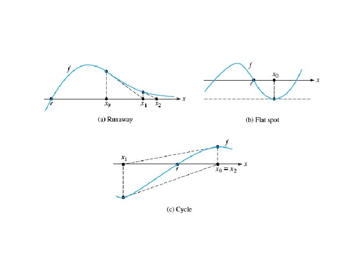
• Newton’s method convergence depends upon hypotheses difficult to verify a priori • graphical examples • the tangent to the graph of the function f at x 0 intersects the x-axis at a point remote from the root r, • and successive points in Newton’s iteration – recede from r instead of converging to r. • poor choice of the initial point x 0; • it is not sufficiently close to r

• In (b): • the tangent to the curve: • parallel to the x-axis and x 1 = ∞, or it is assigned the value of machine infinity in a computer.

• In part (c) • the iteration values cycle because x 2 = x 2 • In a computer – roundoff errors – or limited precision • may eventually cause this situation to become unbalanced • such that the iterates either – spiral inward and converge – or spiral outward and diverge.

Quadratic Convergence • • • the quadratic convergence another troublesome hypothesis; f’(r ) = 0. r is a zero of f and f’. multiple zero of f —at least a double zero Newton’s iteration for a multiple zero converges only linearly! • not known in advance: • zero sought was a multiple zero

• If multiplicity is knownt – m • Newton’s method - accelerated by modifying the equation: • • m: the multiplicity of the zero The multiplicity of the zero r : the least m such that f (k)(r ) = 0 for 0 k < m but f (m) (r ) 0

• • • p 2(x) = x 2 − 2 x + 1 = 0 root at 1 of multiplicity 2 p 3(x) = x 3 − 3 x 2 + 3 x − 1 = 0 root at 1 of multiplicity 3 plot these curves rather flat at the roots slows down the convergence of the regular Newton’s method the curves of two nonlinear functions with multiplicities as well as their regions of uncertainty about the curves. the computed solutions could be anywhere within the indicated intervals on the x-axis indication of the difficulty in obtaining precise solutions of nonlinear functions with multiplicities.

Curves p 2 an p 3 wit multiplicit 2 and 3

Systems of Nonlinear Equations • Some problems solution of systems of N nonlinear equations in N unknowns • One approach - linearize and solve, repeatedly – same strategy used by Newton’s method in solving a single nonlinear equation • a natural extension of Newton’s method for nonlinear systems • some familiarity with matrices and their inverses

• a system of N nonlinear equations in N unknowns x i: • Using vector notation: F(X) = 0 • defining column vectors as

• The extension of Newton’s method for nonlinear systems is • where F’ (X(k)): the Jacobian matrix • partial derivatives of F evaluated at X(k) = [x(k)1 , x(k)2, . . . , x(k)N ]T.

• similar to the previously seen version of Newton’s method – except the derivative expression is notin the denominator but in the numerator as the inverse of a matrix • In the computational form of the formula X(0) = [x(0)1 , x(0)2, . . . , x(0)N ]T • is an initial approximation vector – taken to be close to the solution of the nonlinear system – and the inverse of the Jacobian matrix is not computed but rather a related system of equations is solved

• illustrate the development of this procedure using three nonlinear equations • the Taylor expansion in three variables for i = 1, 2, 3: • where the partial derivatives are evaluated at the point (x 1, x 2, x 3) • only the linear terms in step sizes hi are shown.

• Suppose that the vector • X(0) = = (x(0)1 , x(0)2, . . . , x(0)N )T • an approximate solution to the systems of equations. • Let H = [h 1, h 2, h 3]T • be a computed correction to the initial guess so that X(0) +H = [x(0)1+h 1, x(0)2+h 2, x(0)3+h 3 ]T • better approximate solution. • Discarding the higher-order terms in the Taylor expansion , in vector notation:

• where the Jacobian matrix is defined by • all partial derivatives evaluated at X(0): • assume that the Jacobian matrix F’(X(0)) – nonsingular - its inverse exists.

• Solving for H: • Let X(1) = X(0) + H - better approximation after the correction; • arrive at the first iteration of Newton’s method for nonlinear systems • In general, Newton’s method uses this iteration:

• In practice, the computational form of Newton’s method does not involve • inverting the Jacobian matrix • but rather solves the Jacobian linear systems • The next iteration of Newton’s method: • Newton’s method for nonlinear systems • The linear system can be solved by procedures Gauss and Solve • Small systems of order 2 can be solved easily

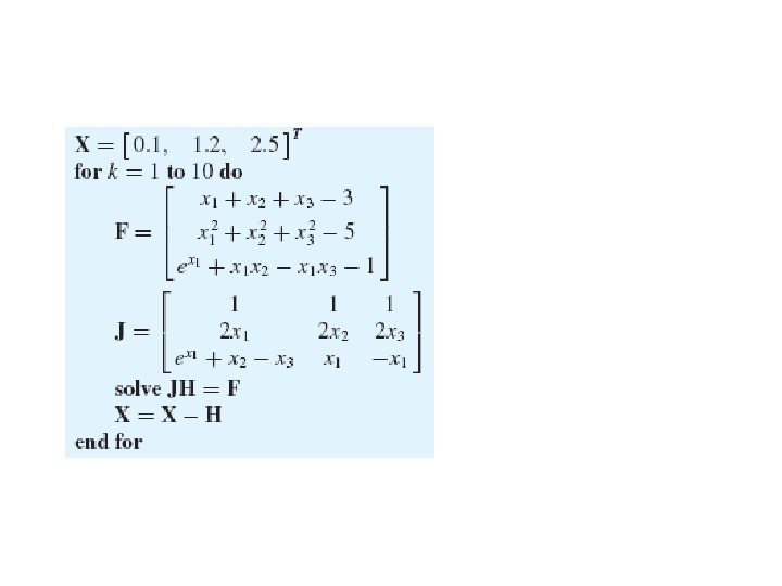
Example • write a pseudocode to solve the following nonlinear system of equations using a variant of Newton’s method

Solution • the solution of this system: x = 0, y = 1, z = 2 • most realistic problems, solution not obvious • develop a numerical procedure for finding such a solution

Pseudocode • use mathematical software such as in Matlab, Maple, or Mathematica • and their built-in procedures • for solving the system of nonlinear equations • An important application area of solving systems of nonlinear equations is on minimization of functions.

• • When programmed and executed, it converges to x = (0, 1, 2) but change to a different starting vector, (1, 0, 1), it converges to another root: (1. 2244, − 0. 0931, 1. 8687)

Secant Method

Secant method • general-purpose procedure - converges almost as fast as Newton’s method • mimics Newton’s method but avoids the calculation of derivatives. • Newton’s iteration defines: • In secant method replace f’(xn) by an approximation – easily computed • derivative defined by: • for small h

• finite difference approximation to the first derivative • if x = xn and h = xn− 1 − xn, • When used in Newton’s equation - defines the secant method: • secant method (like Newton’s) used to solve systems of equations as well.

• The name of the method: • the right member in the secant equation - slope of a secant line to the graph of f • the left member - slope of a tangent line to the graph of f • Similarly, Newton’s method - “tangent method. ”

Secant Method

Remartks • xn+1 depends on two previous elements of the sequence • to start, two points (x 0 and x 1) must be provided. secnat equation - generate x 2, x 3, . . • programming the secant method – calculate and test the quantity f (xn)− f (xn-1) • If nearly zero, – an overflow can occur • if the method is succeeding • the points xn will be approaching a zero of f • so f (xn) - converging to zero

• Also, f (xn− 1) will be converging to zero, and, a fortiori, f (xn)− f (xn− 1) will approach zero. • If f (xn) and f (xn− 1) same sign – additional significant digits are canceled in the subtraction • halt the iteration when | f (xn) − f (xn− 1)| δ| f (xn− 1)| – for some specified tolerance δ, such as (½) × 10− 6

Secant Algorithm • A pseudocode for nmax steps of the secant method applied to the function f • starting with the interval [a, b] = [x 0, x 1]: procedure Secant( f, a, b, nmax, ε) integer n, nmax; real a, b, fa, fb, ε, d external function f fa ← f (a) fb ← f (b) if |fa| > |fb| then a ←→ b f a ←→ fb end if

output 0, a, fa output 1, b, fb for n = 2 to nmax do if |fa| > |fb| then a ←→ b fa ←→ f b end if d ← (b − a)/(fb − fa) b←a fb←fa d ← d · fa

if |d| < ε then output “convergence” return end if a←a−d f a ← f (a) output n, a, f a end for end procedure Secant

• ←→: interchange values • The endpoints [a, b] are interchanged – if necessary, to keep | f (a)| | f (b)| • the absolute values of the function are nonincreasing; • | f (xn)| | f (xn+1)| for n 1

Example • If the secant method is used on p(x) = x 5 + x 3 + 3 with x 0 = − 1 and x 1 = 1, what is x 8?

• The output corresponding to the pseudocode for the secant method: (for a 32 -bit word-lengtcomputer) • by a mathematical software - the single real root, − 1. 1053, and the two pairs of complex roots: • − 0. 319201 ± 1. 35008 i and 0. 871851 ± 0. 806311 i

Comparision of Methods • three primary methods for solving an equation f (x) = 0. – The bisection method - reliable but slow – Newton’s method - fast but often only near the root and requires f’ – The secant method - nearly as fast as Newton’s method • not require derivative f’, • may not be available • or may be too expensive to compute • in bisection method - provide two points at which the signs of f (x) differ, and the function f need only be continuous. • Newton’s method - specify a starting point near the root, and f must be differentiable. • secant method - two good starting points

• Newton’s procedure interpreted as – the repetition of a two-step procedure summarized by the prescription – linearize and solve • This strategy applicable in many other numerical problems, • Both Newton’s method and the secant method fail to bracket a root • The modified false position method can retain the advantages of both methods.

• The secant method is often faster at approximating roots of nonlinear functions in • comparison to bisection and false position • Unlike these two methods, the intervals [ak , bk] – do not have to be on opposite sides of the root – and have a change of sign. • Moreover – the slope of the secant line can become quite small – and a step can move far from the current point • The secant method can fail to find a root of a nonlinear function that has a small slope near the root – because the secant line can jump a large amount.

• For nice functions and guesses relatively close to the root, • most of these methods require relatively few iterations before coming close to the root • However, there are pathological functions – cause troubles for any of those methods • When selecting a method for solving a given nonlinear problem • consider many issues such as – – – the behavior of the function an interval [a, b] satisfying f (a) f (b) < 0 the first derivative of the function a good initial guess to the desired root and so on.

Hybrid Methods • to find the best algorithm for finding a zero of a given function, • various hybrid methods have been developed. • Some of these procedures combine the bisection method (used during the early iterations) with either the secant method or the Newton method. Also, adaptive schemes are used for monitoring the iterations and for carrying out stopping rules. • See references

Fixed Point Iteration • • For a nonlinear equation f (x) = 0 seek a point where the curve f intersects the x-axis (y = 0) An alternative approach is to recast the problem as a fixed-point problem x = g(x) for a related nonlinear function g • For the fixed point problem, seek a point where the – curve g intersects the diagonal line y = x • A value of x such that x = g(x) is a fixed point of g – x is unchanged when g is applied to it

• Many iterative algorithms for solving a nonlinear equation f (x) = 0 - based on a fixed-point iterative method x(n-1) = g(x(n)) • where g has fixed points that are solutions of • f (x) = 0. • An initial starting value x(0) is selected, and the iterative method is applied repeatedly until it converges sufficiently well.

Example • Apply the fixed-point procedure, where g(x) 1+2/x, • starting with x(0) = 1, to compute • a zero of the nonlinear function f (x) = x 2 − x − 2. Graphically, trace the convergence process

Solution • The fixed-point method is • Eight steps of the iterative algorithm are x(0) = 1, x(1) = 3, x(2) = 5/3, x(3) = 11/5, • x(4) = 21/11, x(5) = 43/21, x(6) = 85/43, x(7) = 171/85, and x(8) = 341/171 ≈ 1. 99415. • these steps spiral into the fixed point 2.

Fixed poin iterations for f (x) = x 2−x− 2

• • • For a given nonlinear equation f (x) = 0 there may be many equivalent fixed-point problems x g(x) with different functions g, some better than others simple way - characterize the behavior of an iterative method x(n+1) = g(x(n)) locally convergent for x* if x* = g(x*) and |g’(x*)| < 1 By locally convergent: there is an interval containing x(0) such that the fixed-point method converges for any starting value x(0) within that interval If |g’(x*)| > 1, then the fixed-point method diverges for any starting point x(0) other than x*.

• Fixed-point iterative methods are used in standard practice for solving many • science and engineering problems. • In fact, the fixed-point theory can simplify the proof of the convergence of Newton’s method.