CSE 551 Computational Methods 20182019 Fall Chapter 9

CSE 551 Computational Methods 2018/2019 Fall Chapter 9 -A Ordinary Differential Equations

Outline Taylor Series Methods Runge-Kutta Methods Stability and Adaptive Runge-Kutta and Multistep Methods

References • W. Cheney, D Kincaid, Numerical Mathematics and Computing, 6 ed, • Chapter 10

Taylor Series Methods • Initial-Value Problem: Analytical versus Numerical Solution • Solving Differential Equations and Integration • Taylor Series Methods • Taylor Series Method of Higher Order • Types of Errors

Initial-Value Problem: Analytical versus Numerical Solution • An ordinary differential equation (ODE) • equation - one or more derivatives of an unknown function • A solution - differential equation – specific function - satisfies the equation

Examples – t - independent variable – x - dependent variable. – name of the unknown function of the independent variable t: • c - an arbitrary constant

• a DE not, in general, • not determine a unique solution function • accompanied by auxiliary conditions – together with the DE • specify the unknown function precisely.

Inıtial-Value Problem • initial-value problem for a first-order DE. • x - function of t, • (1): initial-value problem • t - time and t = a - initial instant in time. • determine the value of x at any time t before or after a.

Examples • examples of initial-value problems, with solutions: • A numerical solution DE • table; • functional form of the solution remains unknown

• • function f – depend on t and x If f not involve x, - second example – DE solved - indefinite integration. illustrate, • C - x(5) = 17. C = 4 ln(5) − arctan(5) − 108.

• numerical solution DE: • (a) the closed form solution may be very complicated and difficult to evaluate or • (b) there is no other choice; that is, no closed-form solution can be found • e. g. , for the DE • • • solution - taking the integral of the right-hand side. can be done in principle but not in practice. a function x exists dx/dt - right-hand member (3) but it is not possible to write x(t) in terms of familiar functions. .

• Solving ODEs on a computer • require a large number of steps with small step size, • significant amount of roundoff error can accumulate. – multiple-precision computations may be necessary on small-word-length computers.

Solving Differential Equations and Integration • close connection between – solving DEs and integration • e. g. : • Integrating from t to t + h,

• Replacing the integral - numerical integration rules formula for solving the differential equation. • Euler’s method - obtained from the left rectangle approximation • The trapezoid rule

• Since x(t + h) appears on both sides of this equation, it is called an implicit formula. If • Euler’s method • x(t + h) on the right-hand side, then we obtain the Runge-Kutta formula of • order 2—namely, Equation (10) in Section 10. 2.

• Fundamental Theorem of Calculus, • approximate numerical value for the integral • can be computed by solving the following initialvalue problem for x(b):

Taylor Series Methods • represent the solution of a DE locally by a few terms of its Taylor series. • assume that • solution function x - represented Taylor series:

• • • numerical purposes, Taylor series truncated after m+1 terms compute x(t + h) rather accurately h is small and x(t), x’’(t), . . . , x(m)(t) - known. When terms through hmx(m)(t)/m! included in the Taylor series, the method • Taylor series method of order m.

Euler’s Method Pseudocode • Taylor series method of order 1 - Euler’s method • approximate values of the solutions to the initialvalue problem: • over the interval [a, b], • first two terms - Taylor series (5) : • the formula:

• can be used to step from t = a to t = b with n steps of size h = (b−a)/n. • The pseudocode can be written as follows, where some prescribed values for n, a, b, and • xa are used:

pseudocode for Euler’s method

Example 1 • Using Euler’s method, compute an approximate value for x(2) • for the differential equation x’ = 1 + x 2 + t 3 • with the initial value x(1) = − 4 • using 100 steps.

Solution • Use the pseudocode above with the initial values given and combine with the following function: • The computed value is x(2) ≈ 4. 23585

• computer program - execute Euler’s method • simple problem: • • x(2) ≈ 7. 3891. The solution, x(t) = et , points produced by Euler’s method - dots. why the dots are always below the curve?

Euler’s metho curves 0

• some questions such as: • How accurate are the answers? • Are higher-order Taylor series methods ever needed? • Euler’s method - not very accurate • only two terms in the Taylor series (5) –used • truncation error is O(h 2).

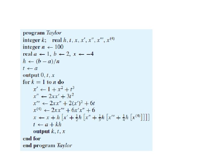
Taylor Series Method of Higher Order • Example 1: • Taylor series method of higher order. • initial-value problem: • functions DE differentiated several times with respect to t (chain rule):

• • • numerical values of t and x(t) known, x’(t), x’’’(t), and x(4)(t) first five terms - Taylor series (5) x(1) = − 4, suitable starting point, n = 100 – h. approximation - x(a + h) - from (5) and (8) same process - repeated compute: x(a + 2 h) form x’(a + h), x’’(a + h), . . . , x(4)(a + h).

• • determine - interval a = 1 t 2 = b, and 100 steps. In each step, current value of t – integer multiple of the step size h. • The assignment statements that • define x’, x’’’, and x(4) carrying out calculations of the derivatives according • to (8)

• evaluation of the TS in (5) – five terms. polynomial in h, • nested multiplication, • The computation t ← t + h – may cause a small amount of roundoff error to accumulate in the value of t • avoided by using t ← a + kh.

• two terms in TS (Euler’s method) not accurate five terms : • Euler’s Method TS Method (Order 4) • x(2) ≈ 4. 23585 41 x(2) ≈ 4. 37120 96 • correct value to more significant figures: • x(2) ≈ 4. 37122 1866 • computations were done with more precision – show that lack of precision was not a contributin factor.

Types of Errors • • • what sort of accuracy expected? Are all the digits for the variable x accurate? not! not easy to say - how many digits are reliable a coarse assessment: Since terms up to (1/24)h 4 x(4)(t) included, first term not included in TS: (1/120) h 5 x(5)(t). The error may be larger than this, but the factor h 5 = (10− 2)5 ≈ 10− 10 affecting only the tenth decimal place.

Trancation Error • • two types of errors At each step, if x(t) known and x(t+h) computed from the first fewterms of the Taylor series, an error occurs truncated the. Taylor series truncation error - local truncation error. In the example, roughly (1/120) h 5 x(5)(ξ ). local truncation error of order h 5 - O(h 5).

Accumulaed Error • The second type of error • accumulated effects of all local truncation errors • calculated value of x(t +h) - in error • x(t) is already wrong – previous truncation errors – another local truncation error occurs in the computation of x(t + h)

Roundoff error • Additional sources of errors: • roundoff error – not serious in any one step of the solution procedure, – after hundreds or thousands of steps, – accumulate and contaminate the calculated solution seriously. • an error - made at a certain step • carried forward into all succeeding steps

Runge-Kutta Methods • Taylor Series for f(x, y) • Runge-Kutta Method of Order 2 • Runge-Kutta Method of Order 4

Runge-Kutta Methods • imitate the Taylor series method • without analytic differentiation of the original DE. • Taylor series method on the initial-value problem

RK method of order 2 • need to obtain x, x’ , . . . • differentiating the function f. – serious obstacle • a method for solving (1) – writing a code to evaluate f • • The Runge-Kutta (RK) methods. RK method of order 2 low precision RK method of order 4 - common use.

Hearth of an IV Problem • • • heart of - initial-value problem advancing the solution function one step at a time; formula for x(t + h) - known quantities x(t), x(t − h), x(t − 2 h), . . . At the beginning, only x(a) is known.

Taylor Series for f(x, y) • Taylor series in two variables: • f and all partial derivatives evaluated at (x, y)

• Taylor series - truncated • error term or remainder term - restore the equality: • point (xb, yb) lies on the line segment – joins (x, y) to (x + h, y + k) in the plane • subscripts - denote partial derivatives.

• functions - order of subscripts immaterial; • e. g. fxt = ftx. • special cases:

Runge-Kutta Method of Order 2 • Runge-Kutta method of order 2 - a formula: • two function evaluations of the special form • linear combination of these - added to the value of x at t - at t +h:

• determine constants w 1, w 2, α, and β – (5) as accurate as possible • reproduce as many terms as possible in the TS

• • • compare (5) with (6). One way to force them to agree up through the term in h - set w 1 = 1 and w 2 = 0 x=f. Euler’s method - order of precision is only 1. Agreement up through the h 2 term is possible by a more adroit choice of parameters. • apply two-variable form TS - final term in (5). – n = 2 - two-variable TS Formula (3), – with t, αh, x, and βh f – playing the role of x, h, y, and k, respectively:

• new form for (5):

• Equation (6) - new form by using DE (1). • x’ = f , • (6) implies that • Agreement between (7) and (8)

• solution • The resulting second-order Runge-Kutta method is then, from Equation (5), : • equivalently,

• (10) - solution function at t + h – – two evaluations of the function f • other solutions - nonlinear System (9) possible. • For example, α can be arbitrary,

Error Term • error term for R-K methods of order 2: • none of the secondorder • RK methods - widely used • error O(h 3).

Runge-Kutta Method of Order 4 • algorithm – IV Problem (1) • fourth-order Runge-Kutta method.

About Error • solution at x(t + h) obtained • evaluating the function f four times • The final formula agrees with the Taylor expansion up to and including the term in h 4 • The error contains h 5 – no lower powers of h. • Without knowing the coefficient of h 5 in the error, – cannot be precise about the local truncation error.

Pseudocode

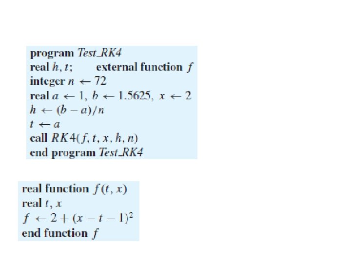
Illustration • illustrate use of pseudocode, • IV problem • exact solution: x(t) = 1 + tan(t − 1). • on the interval [1, 1. 5625] RK procedure: • step size: – dividing the length of the interval by the number of steps, say, n = 72.

• The final value of the computed numerical solution: • x(1. 5625) = 3. 19293 7699.

Software • • • General-purpose routines RK algorithm monitor - truncation error make necessary adjustments step size as the solution progresses. In general terms, the step size – can be large when the solution is slowly varying – but should be small when it is rapidly varying.

Stability and Adaptive Runge-Kutta and Multistep Methods • An Adaptive Runge-Kutta-Fehlberg Method • An Industrial Example • Adams-Bashforth-Moulton Formulas

An Adaptive Runge-Kutta-Fehlberg Method • numerical solution of initial-value problems, – estimate the precision attained in the computation. • error tolerance • the numerical solution must not deviate from the true solution beyond this tolerance. • error tolerance - largest allowable step size – local truncation error, • determining appropriate step size – difficult – small step size - on one portion of the solution curve, – larger one - uffice elsewhere.

An Adapteive Procedure • methods for automatically adjusting the step size IV problem. • One simple procedure: • fourth-order RK method. • To advance the solution curve from t to t + h, one step of size h • RK formulas • two steps of size h/2 to arrive at t + h • If no truncation error: • x(t + h) would be the same for both procedures • difference numerical results – – estimate of the local truncation error

An Adapteive Procedure • • • if this difference - within the prescribed tolerance the current step size h is satisfactory If this difference exceeds the tolerance the step size is halved If the difference is very much less than the tolerance, the step size is doubled.

Fehlberg Method of Order 4 • The procedure - not recommended. • A more sophisticated method by Fehlberg • Fehlberg method of order 4 – RK type and uses these formulas:

Fehlberg Method of Order 4 (cont. ) • requires one more function evaluation than the classical RK method of order 4, – questionable value alone.

• additional function evaluation • fifth-order Runge-Kutta method

• The difference between the values of x(t + h) • obtained from the fourth- and fifth-order procedures • estimate of the local truncation error • fourth-order procedure • six function evaluations – • fifth-order approximation, – together with an error estimate!

pseudode RK 45

pseudode RK 45 (cont. )

Non Adaptive Use of RL 45

• • print the error estimation at each step. can use it in an adaptive procedure, error estimate ε - when to adjust the step size to control the single-step error.

A Simple Adaptive Process • In the RK 45 procedure, the fourth- and • fifth-order approximations for x(t + h), say, x 4 and x 5, are computed from six function evaluations, • and the error estimate ε = |x 4 − x 5| is known. • From user-specified bounds on the allowable error estimate – (εmin ε εmax), • • • the step size h is doubled or halved as needed to keep ε within these bounds. A range for the allowable step size h is also specified by the user (hmin |h| hmax). the user must set the bounds (εmin, εmax, hmin, hmax) carefully – the adaptive procedure does not get caught in a loop, – trying repeatedly to halve and double the step size from the same point – to meet error bounds that are too restrictive for the given differential equation.

• adaptive process :

Parameter List • • The procedure - RK 45 Adaptive. parameter list f: function f (t, x) for the DE, t and x : contain the initial values, h: the initial step size, tb: the final value for t, itmax: the maximum number of steps to be taken in going from a = ta to b = tb, • εmin and εmax: lower and upper bounds on the allowable error estimate ε, • hmin and hmax: bounds on the step size h,

Parameter List (cont. ) • and iflag: an error flag that returns one of the following values: • • iflag Meaning 0 Successful march from ta to tb 1 Maximum number of iterations reached On return, t and x are the exit values, and h is the final step size value considered or used:

• • In the pseudocode, several conditions must be checked to determine the size of the final step, floating-point arithmetic is involved and the step size varies.

An Industrial Example • A first-order DE arose in the modeling of an industrial chemical process : • • • a = 3, b = 5, and c = 0. 2 are constants. adaptive RK formulas, identify (and program) the function f f (t, x) = 3 + 5 sin t + 0. 2 x. brief pseudocode for solving the equation on the interval [0, 10] – particular values assigned to the parameters in the routine RK 45 Adaptive:

• obtain approximation: x(10) ≈ 135. 917

Adams-Bashforth-Moulton Formulas • strategy - numerical quadrature formulas • solve single first-order ODE. • the values of the unknown function computed at several points to the left of t, – t, t − h, t − 2 h, . . . , t − (n − 1)h • compute x(t + h).

• theorems of calculus: • abbreviation: f j = f (t − ( j − 1)h, x(t − ( j − 1)h))

• numerical integration formula. • simplest case - for the interval [0, 1] • use values of the integrand at points 0, − 1, − 2, . . . , 1−n – in the case of an Adams-Bashforth formula. • basic rule - change of variable • the rule any other interval with any other uniform spacing.

• a rule of the form • • • n coefficients cj at our disposal. interpolation theory formula - exact for all polynomials of degree n − 1. integrating each function 1, r, r 2, . . . , r n− 1 exactly. appropriate equation:

• • • system Au = b n equations in n unknowns Ai j = (1 − j )i− 1, bi = 1/i. output: vector of coefficients ( 55/24 , − 59/24 , 37/24 , − 3/8). higher-order formulas by changing the value of n in the code. • Adams-Moulton formulas, start with a quadrature rule of the form

• tt+h 01 • A program similar to the one above yields the coefficients • 9/24 , 19/24 , − 5/24 , 1/24 • The distinction between the two quadrature rules is that one involves the value of the integrand at 1 and the other does not.

• How do we arrive at formulas for • tt+h g(s) ds from the work already done? • Use the change of variable from s to σ given by s = hσ − t. • In these considerations, think of t as a constant • The new integral: 01 g(hσ + t) dσ, • treated with either of the two formulas already designed for the interval [0, 1]. For example,

• method of undetermined coefficients • obtain the quadrature formulas does • not, by itself, provide the error terms that we would like to have. • assessment of the error - interpolation theory, – integrating an interpolating polynomial

CSE 551 Computational Methods 2018/2019 Fall Chapter 9 -B Systems of Ordinary Differentia Equations

Outline Methods for First-Order Systems Higher-Order Equations and Systems Adams-Bashforth-Moulton Methods

References • W. Cheney, D Kincaid, Numerical Mathematics and Computing, 6 ed, • Chapter 11

Methods for First-Order Systems • • Uncoupled and Coupled Systems Taylor Series Method Vector Notation Systems of ODEs Taylor Series Method: Vector Notation Runge-Kutta Method Autonomous ODE

Methods for First-Order Systems • ODEs – single DE, first order – with an accompanying auxiliary condition. • systems of several first-order equations.

Uncoupled and Coupled Systems • The sun and the nine planets - system of particles – Newton’s law of gravitation • • • position vectors of the planets system of 27 functions, and the Newtonian laws of motion system of 54 first-order ODEs In principle, – past and future positions of the planets can be obtained by solving these equations numerically.

Example • two equations with two auxiliary • conditions • x and y be two functions of t: • with initial conditions

• initial-value problem - system of two first-order DEs. • not possible - solve – either of the two DEs by itself – first equation governing x involves the unknown function y, – and the second equation governing y involves the unknown function x. • two DEs - coupled. • analytic solution:

• simpler example: • initial conditions: • not coupled • solved separately - two unrelated initialvalue problems

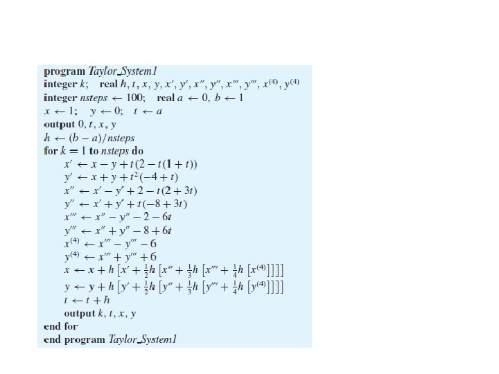
Taylor Series Method • Taylor series (TS) method for System (1) • differentiating the equations :

• program to proceed – from x(t) to x(t + h) – and from y(t) to y(t + h) • few terms of the Taylor series: • together with equations for the various derivatives. • x and y and all their derivatives - functions of t; • x = x(t), y = y(t), x’ = x’(t), y’ = y’(t), and so on.

• • • A pseudocode program generates and prints a numerical solution from 0 to 1 in 100 steps: Terms up to h 4 have been used in the Taylor series.

Vector Notation • (1) vector notation: • initial conditions

• more general problem: • where • F vector two components right-hand sides in (1). • depends on t and X, - F(t, X).

Systems of ODEs • ystem of n first-order differential equations. • (4), ODE in vectornotation.

Taylor Series Method: Vector Notation • m-order Taylor series method • X = X(t), X’ = X’(t), X’’ = X’’(t), and so on.

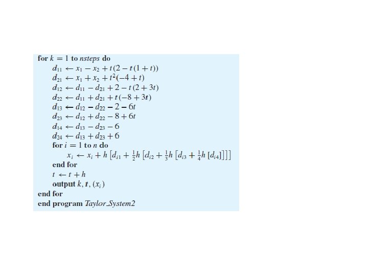
• • pseudocode TS method - order 4 preceding problem simple change of variables an array and, inner loop.

• • a two-dimensional array instead of all the different derivative variables; di j ↔ xi( j ). easy to program – computer language supports vector operations.

Runge-Kutta Method • RK extend to systems of DEs. • fourth-order RK method for (4): • where • X = X(t), and all quantities are vectors with n components except variables t and h.

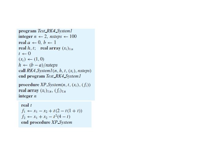
• A procedure Runge-Kutta procedure • system to be solved - (4) n equations in • The user furnishes: – – initial value of t, the initial value of X, the step size h, and the number of steps to be taken, nsteps. • procedure XP System(n, t, (xi ), ( fi )) – needed: – evaluates the right-hand side of (4) for a given value of array (xi ) – stores the result in array ( fi ).

pseudocode RK 4_System 1

pseudocode RK 4_System 1

pseudocode RK 4_System 1

Illustration • illustrate use of this procedure, • use System (1) for example. • rewritten in the form of (4)

• A numerical experiment: • compare the results of the TS method and the • RK method with the analytic solution of System (1) • At the point t = 1. 0, the results : • TS RK AS • x(1. 0) ≈ 2. 46869 40 2. 46869 42 2. 46869 39399 • y(1. 0) ≈ 1. 28735 46 1. 28735 61 1. 28735 52872

• use mathematical software routines found in Matlab, Maple, or Mathematica to • obtain the numerical solution of the system of ordinary differential equations (1) • For t over • the interval [0, 1], invoke an ODE procedure to march from t = 0 at which x(0) = 1 • and y(0) = 0 to t = 1 at which x(1) = 2. 468693912 and y(1) = 1. 287355325. • To obtain the numerical solution of the ordinary differential equation defined for t over • the interval [1, 1. 5], invoke an ordinary differential equation solving procedure to march • from t = 0 at which x(1) = 2 and y(1) = − 2 to t = 1. 5 at which x(1. 5) ≈ 15. 5028 and • y(1. 5) ≈ 6. 15486.

Autonomous ODE • system of differential equations in vector form • variable t - explicitly separated from the other variables • new variable x 0 is t in disguise • add a new DE x’ 0 = 1. • a new initial condition x 0(a) = a. • increase # of DEs from n to n + 1

• system in vector form: • system of two equations given by (1). • system with three variables:

• auxiliary condition for X : • X(0) = [0, 1, 0]T. • a system of n + 1 first-order differential equations

• in general vector notation:

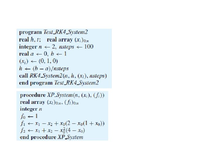
• A system of DEs without the t variable explicitly present autonomous. • numerical methods not require • x 0 = t or f 0 = 1 or s 0 = a. • For an autonomous system, the classical fourthorder Runge-Kutta method for System (6) uses these formulas: • X = X(t),

• procedure RK 4 System 1 modified: • beginning the arrays with 0 rather than 1 • and omitting the variable t.

Higher-Order Equations and Systems • Higher-Order Differential Equations • Systems of Higher-Order Differential Equations • Autonomous ODE Systems

Higher-Order Equations and Systems • initial-value problem for ODEs of order higher than 1. • A DE of order n - n auxiliary conditions • initial conditions are needed to specify the solution of the differential equation precisely • e. g. , a particular second-order initial-value problem:

• Without the auxiliary conditions, the general analytic solution: • • • c 1 and c 2 - arbitrary constants To select one specific solution, c 1 and c 2 fixed, two initial conditions x(0) = 0 - c 2 = − 3/8 , and x’(0) = 0 forces c 1 = 0.

Higher-Order Differential Equations • general form of an ODE with initial conditions • solved numerically - turning it into a system of first-order differential equations. • define new variables x 1, x 2, . . . , xn:

• original initial-value problem (2) equivalent to

• in vector notation,

• problem - transformed - new variables, • dictionary – relationship between the new and the old variables • illustration: • into a form - solution by the Runge-Kutta procedure.

• A chart summarizing the transformed problem: • corresponding first-order system: • X(0) = [3, 7, 13]T.

Systems of Higher-Order Differential Equations • introducing new variables, • transform a system of DEs of various orders into a larger system of first-order equations • e. g. , • solved by Runge-Kutta procedure

• transform: • X(1) = [2, − 4, − 2, 7, 6]T.

Autonomous ODE Systems • t present on the right-hand side of (3) • x 0 = t and x 0 ’ = 1 introduced to form an autonomous system of ODEs in vector notation.

• a higher-order system of DEs (2) • written in vector notation as

Example • the ODE system in (4) in autonomous form: • X(1) = [1, 2, − 4, − 2, 7, 6]T.

Adams-Bashforth-Moulton Methods • A Predictor-Corrector Scheme

A Predictor-Corrector Scheme • initial-value problem • single-step numerical methods • if X(t) – known at t, • X(t + h) computed – no knowledge at points earlier than t • RK and TS methods: – compute X(t + h) in terms of X(t) and various values of F.

• More efficient methods – X(t), X(t −h), X(t − 2 h), . . . • computing X(t + h) • multistep methods. • drawback: at the beginning of the numerical solution, • no prior values of X are available • start - single-step method, such as RK, • transfer - multistep procedure – enough starting values computed.

• a multistep formula - Adams-Bashforth method

• • Xb (t + h) - predicted value of X(t + h) computed by (2). solution X computed at four points t, t − h, t − 2 h, t − 3 h (2) used to compute X (t + h) one evaluation of F - required for each step. considerable savings over the fourth-order RK procedure; four evaluations of F per step. consideration of truncation error and stability – permit a larger step size in RK method – and make it much more competitive

Corrector • • (2) not used by itself predictor, another formula – corrector Adams-Moulton formula: • (2) predicts a tentative value of X(t +h), • (3) computes this X value more accurately • predictor-corrector scheme.

• initial values of X specified at a, • three steps RK method - determine enough X values • ABM procedure can begin • The fourth-order Adams-Bashforth and Adams. Moulton formulas, started with the fourth-order RK method, • Adams-Moulton method. • Predictor and corrector formulas of the same order • only one application of the corrector formula needed

CSE 551 Computational Methods 2018/2019 Fall Chapter 9 -C Boundary-Value Problems for Ordinary Differential Equations

Outline • Shooting Method

References • W. Cheney, D Kincaid, Numerical Mathematics and Computing, 6 ed, • Chapter 14. 1

Shooting Method • A boundary-value problem • exemplified: second-order. ODE • solution function prescribed at the endpoints of the interval

• a DE - general solution involves two arbitrary parameters. • particular solution - two conditions must be given • initial-value problem: – x and x’ specified at some initial point • In this problem: • two points of the form (t, x(t)) - solution curve passes – (0, 1) and (π/2, − 3) • • general solution of DE: x(t) = c 1 sin(t) + c 2 cos(t), two conditions -boundary values determine: c 1 = − 3 and c 2 = 1.

• problem - unable to determine the general solution model the problem: • step-by-step numerical solution (1) • requires two initial conditions • one condition at t = a

• • • guess x’(a), then carry out the solution of IVproblem as far as b, and hope that the computed solution agrees with β; that is, x(b) = β. If not go back and change guess for x’(a) Repeating this procedure until hit the target β good method learn something from the various trials systematic ways of utilizing this information, shooting.

• final value x(b) - solution of initial-value problem • depends on guess for x’(a) • Everything else remains fixed in this problem. Thus, • the differential equation x = f (t, x, x’) and the first initial value, x(a) = α, do not change. • If assign a real value z to the missing initial condition,

• x’(a) = z • then the initial-value problem can be solved numerically. • value of x at b - function of z - ϕ(z) • for each choice of z - obtain a new value for x(b), • and ϕ is the name of the function with this behavior. • know very little about ϕ(z), • but compute or evaluate it. • an expensive function to evaluate – each value of ϕ(z) is obtained only after solving an initialvalue problem.

• shooting method combines • any algorithm for the initial-value problem with • any algorithm for finding a zero of a function

Shootin metho illustrated

Shooting Method Algorithm • a function ϕ(z) is computed: • Solve the initial-value problem • • on the interval [a, b]. Let ϕ(z) = x(b) objective: adjust z until find a value for which ϕ(z) = β linear interpolation between ϕ(z 1) and ϕ(z 2),

• where z 1 and z 2 : – two guesses for the initial condition x’(a). • given two values of ϕ, we pretend that • ϕ is a linear function and determine an appropriate value of z based on this hypothesis. • A sketch of the values of z versus ϕ(z) might look like Figure 14. 3. The strategy just outlined • is the secant method for finding a zero of • ϕ(z) − β.

• To obtain an estimating formula for the next value z 3, we compute ϕ(z 1) and ϕ(z 2) on • the basis of values z 1 and z 2, respectively.

• By similar triangles • repeat this process and generate the sequence • all based on two starting values z 1 and z 2.

• This procedure for solving the two-point boundary -value problem • is then as follows: Solve the initial-value problem

• from t = a to t = b, letting the value of the solution at b be denoted by ϕ(z). Do this twice • with two different values of z, say, z 1 and z 2, and compute ϕ(z 1) and ϕ(z 2). Now calculate a • new z, called z 3, by Formula (2). Then compute ϕ(z 3) by again solving (4). Obtain z 4 from • z 2 and z 3 in the same way, and so on. Monitor

• ϕ(zn+1) − β • to see whether progress is being made. When it is satisfactorily small, stop. This process • is called a shooting method. Note that the numerically obtained values x(ti ) for a ti b • must be saved until better ones are obtained (that is, one whose terminal value x(b) is closer • to β than the present one) because the objective in solving Problem (3) is to obtain va

• x(t) for values of t between a and b. • The shooting method may be very time-consuming if each solution of the associated • initial-value problem involves a small value for the step size h. Consequently, we use a • relatively large value of h until |ϕ(zn+1) − β| is sufficiently small and then reduce h to • obtain the required accuracy.

Example • What is the function ϕ for this two-point boundary -value problem?

Solution • The general solution of the differential equation is x(t) = c 1 et +c 21 e-t. The solution of the • initial-value problem • is

Modifications and Refinements • Many modifications and refinements are possible. For instance, when ϕ(zn+1) is near β, one • can use higher-order interpolation formulas to estimate successive values of zi. Suppose, • for example, that instead of utilizing two values ϕ(z 1) and ϕ(z 2) to obtain z 3, we utilize the • four values • to estimate z 5. set up a cubic interpolatin polynomial p 3 for

• f • nd solve • for z 5. Since p 3 is a cubic, this would entail some additional work. A better way may be to • set up a polynomial p 3 to interpolate the data

• and then use p 3(β) as the estimate for z 5. This procedure is known as inverse interpolation