Computational Complexity Theory Lecture 2 Reductions NPcompleteness CookLevin
- Slides: 117
Computational Complexity Theory Lecture 2: Reductions, NPcompleteness, Cook-Levin theorem Indian Institute of Science
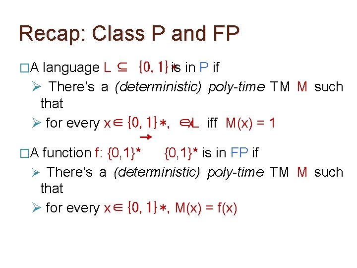
Recap: Class P and FP �A language L ⊆ {0, 1}*is in P if Ø There’s a (deterministic) poly-time TM M such that Ø for every x∈{0, 1}*, ∈L x iff M(x) = 1
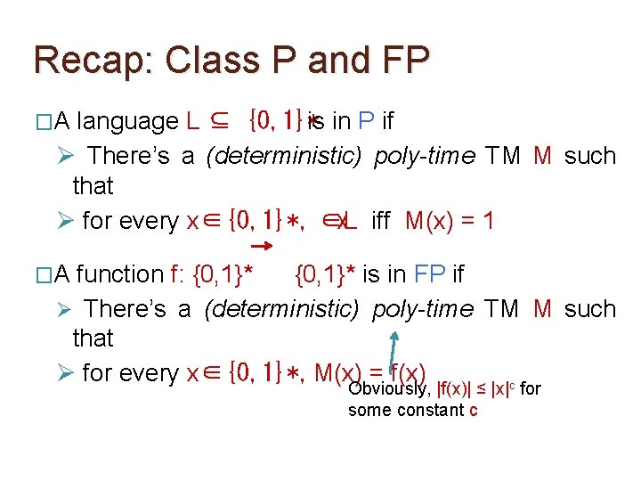
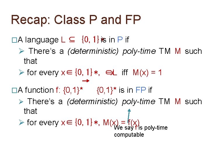
Recap: Class P and FP �A language L ⊆ {0, 1}*is in P if Ø There’s a (deterministic) poly-time TM M such that Ø for every x∈{0, 1}*, ∈L x iff M(x) = 1 �A function f: {0, 1}* is in FP if Ø There’s a (deterministic) poly-time TM M such that Ø for every x∈{0, 1}*, M(x) = f(x)
Recap: Class P and FP �A language L ⊆ {0, 1}*is in P if Ø There’s a (deterministic) poly-time TM M such that Ø for every x∈{0, 1}*, ∈L x iff M(x) = 1 �A function f: {0, 1}* is in FP if Ø There’s a (deterministic) poly-time TM M such that Ø for every x∈{0, 1}*, M(x) = f(x) c Obviously, |f(x)| ≤ |x| for some constant c
Recap: Class P and FP �A language L ⊆ {0, 1}*is in P if Ø There’s a (deterministic) poly-time TM M such that Ø for every x∈{0, 1}*, ∈L x iff M(x) = 1 �A function f: {0, 1}* is in FP if Ø There’s a (deterministic) poly-time TM M such that Ø for every x∈{0, 1}*, M(x) = f(x) We say f is poly-time computable
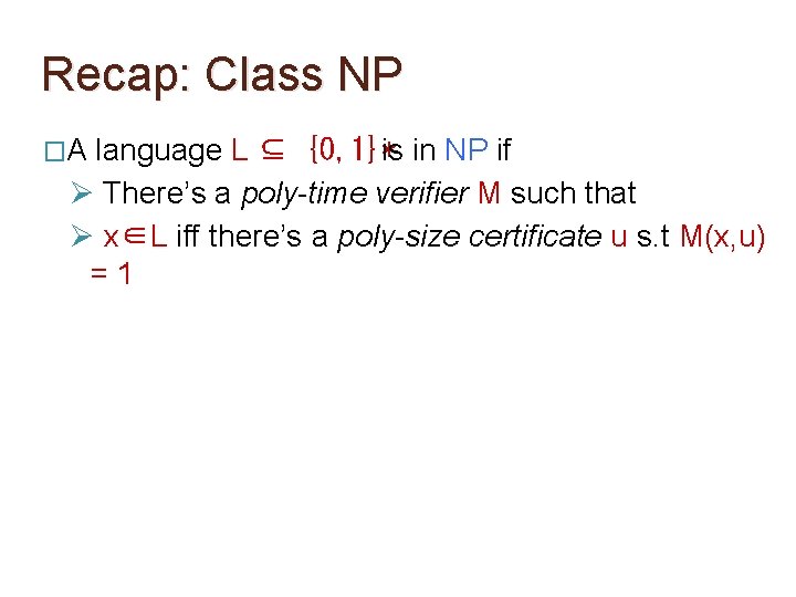
Recap: Class NP �A language L ⊆ {0, 1}*is in NP if Ø There’s a poly-time verifier M such that Ø x∈L iff there’s a poly-size certificate u s. t M(x, u) =1
Recap: Class NP �A language L ⊆ {0, 1}*is in NP if Ø There’s a poly-time verifier M such that Ø x∈L iff there’s a poly-size certificate u s. t M(x, u) =1 Ø Note that verifier cannot be fooled.
Recap: Class NP �A language L ⊆ {0, 1}*is in NP if Ø There’s a poly-time verifier M such that Ø x∈L iff there’s a poly-size certificate u s. t M(x, u) =1 Ø Note that verifier cannot be fooled. � Linear Programming (search version): Given m constraints of the form a 1 x 1 + … + anxn ≤ b where ai’s are rationals, check if there exists an assignment of rational numbers to the xi’s that satisfy all constraints.
Recap: Class NP �A language L ⊆ {0, 1}*is in NP if Ø There’s a poly-time verifier M such that Ø x∈L iff there’s a poly-size certificate u s. t M(x, u) =1 Ø Note that verifier cannot be fooled. � Assignment problem: Programming is in NP. Prove that Linear
Nondeterministic Turing Machines �A nondeterministic Turing machine is like a deterministic Turing machines but with two transition functions. �It is formally defined by a tuple (Γ, Q, δ 0 , δ 1).
Nondeterministic Turing Machines �A nondeterministic Turing machine is like a deterministic Turing machines but with two transition functions. �It is formally defined by a tuple (Γ, Q, δ 0 , δ 1). It has a special state qaccept in addition to qstart and qhalt.
Nondeterministic Turing Machines �A nondeterministic Turing machine is like a deterministic Turing machines but with two transition functions. �It is formally defined by a tuple (Γ, Q, δ 0 , δ 1). It has a special state qaccept in addition to qstart and qhalt. �At every step of computation, the machine applies one of two functions δ 0 and δ 1 arbitrarily.
Nondeterministic Turing Machines �A nondeterministic Turing machine is like a deterministic Turing machines but with two transition functions. �It is formally defined by a tuple (Γ, Q, δ 0 , δ 1). It has a special state qaccept in addition to qstart and qhalt. �At every step of computation, the machine applies one of two functions δ 0 and δ 1 arbitrarily. this is different from randomly
Nondeterministic Turing Machines �A nondeterministic Turing machine is like a deterministic Turing machines but with two transition functions. �It is formally defined by a tuple (Γ, Q, δ 0 , δ 1). It has a special state qaccept in addition to qstart and qhalt. �At every step of computation, the machine applies one of two functions δ 0 and δ 1 arbitrarily. also called nondeterministically
Nondeterministic Turing Machines �A nondeterministic Turing machine is like a deterministic Turing machines but with two transition functions. �It is formally defined by a tuple (Γ, Q, δ 0 , δ 1). It has a special state qaccept in addition to qstart and qhalt. �At every step of computation, the machine applies one of two functions δ 0 and δ 1 arbitrarily. �Unlike DTMs, NTMs are not intended to be physically realizable (because of the arbitrary nature of application of the transition functions).
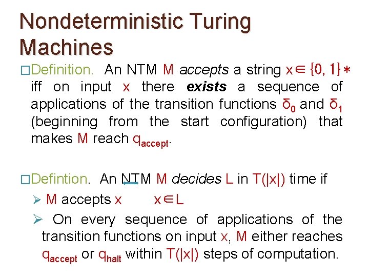
Nondeterministic Turing Machines �Definition. An NTM M accepts a string x∈{0, 1}* iff on input x there exists a sequence of applications of the transition functions δ 0 and δ 1 (beginning from the start configuration) that makes M reach qaccept.
Nondeterministic Turing Machines �Definition. An NTM M accepts a string x∈{0, 1}* iff on input x there exists a sequence of applications of the transition functions δ 0 and δ 1 (beginning from the start configuration) that makes M reach qaccept. �Defintion. An NTM M decides a language L ⊆ {0, 1}* if Ø M accepts x x∈L Ø On every sequence of applications of the transition functions on input x, M either reaches q or q.
Nondeterministic Turing Machines �Definition. An NTM M accepts a string x∈{0, 1}* iff on input x there exists a sequence of applications of the transition functions δ 0 and δ 1 (beginning from the start configuration) that makes M reach qaccept. �Defintion. An NTM M decides a language L ⊆ {0, 1}* if Ø M accepts x x∈L Ø On every remember sequence of applications of the in this course we’ll always be dealing with transition functions on x, M either reaches TMs that halt on input every input. q or q.
Nondeterministic Turing Machines �Definition. An NTM M accepts a string x∈{0, 1}* iff on input x there exists a sequence of applications of the transition functions δ 0 and δ 1 (beginning from the start configuration) that makes M reach qaccept. �Defintion. An NTM M decides L in T(|x|) time if Ø M accepts x x∈L Ø On every sequence of applications of the transition functions on input x, M either reaches qaccept or qhalt within T(|x|) steps of computation.
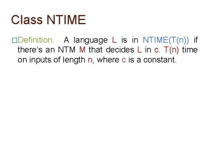
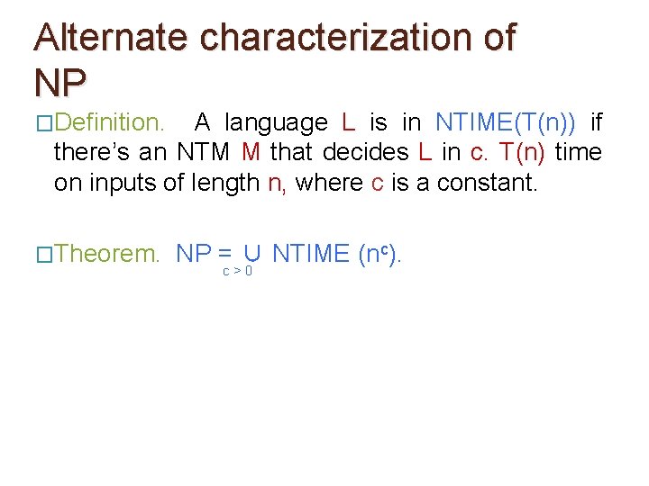
Class NTIME �Definition. A language L is in NTIME(T(n)) if there’s an NTM M that decides L in c. T(n) time on inputs of length n, where c is a constant.
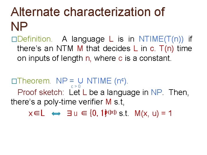
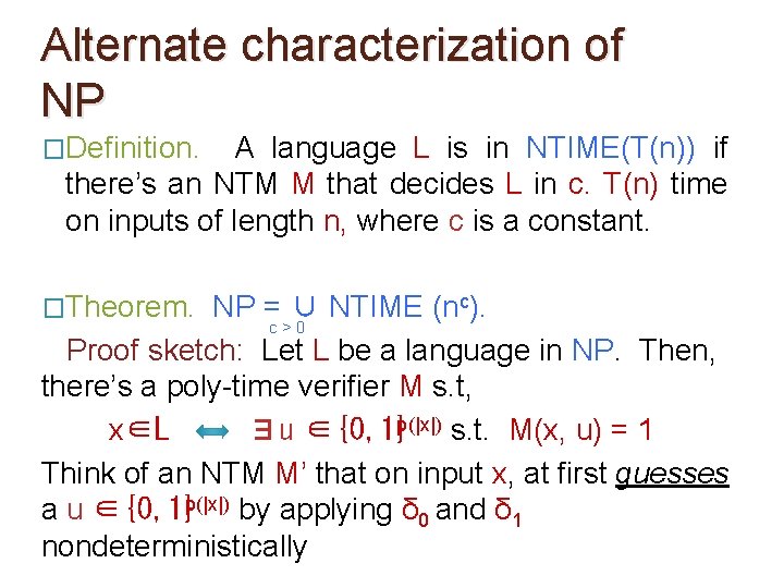
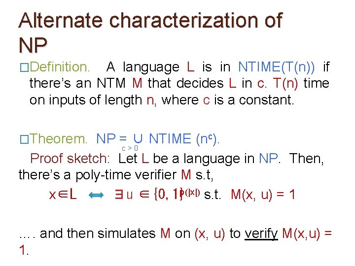
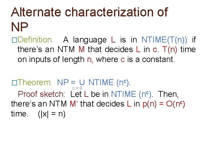
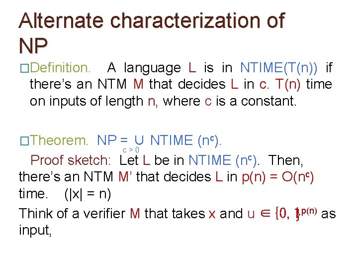
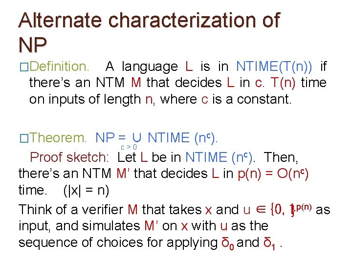
Alternate characterization of NP �Definition. A language L is in NTIME(T(n)) if there’s an NTM M that decides L in c. T(n) time on inputs of length n, where c is a constant. �Theorem. NP = ∪ NTIME (nc). c>0
Alternate characterization of NP �Definition. A language L is in NTIME(T(n)) if there’s an NTM M that decides L in c. T(n) time on inputs of length n, where c is a constant. �Theorem. NP = ∪ NTIME (nc). c>0 Proof sketch: Let L be a language in NP. Then, there’s a poly-time verifier M s. t, x∈L ∃u ∈{0, 1}p(|x|) s. t. M(x, u) = 1
Alternate characterization of NP �Definition. A language L is in NTIME(T(n)) if there’s an NTM M that decides L in c. T(n) time on inputs of length n, where c is a constant. �Theorem. NP = ∪ NTIME (nc). c>0 Proof sketch: Let L be a language in NP. Then, there’s a poly-time verifier M s. t, x∈L ∃u ∈{0, 1}p(|x|) s. t. M(x, u) = 1 Think of an NTM M’ that on input x, at first guesses a u ∈{0, 1}p(|x|) by applying δ 0 and δ 1 nondeterministically
Alternate characterization of NP �Definition. A language L is in NTIME(T(n)) if there’s an NTM M that decides L in c. T(n) time on inputs of length n, where c is a constant. �Theorem. NP = ∪ NTIME (nc). c>0 Proof sketch: Let L be a language in NP. Then, there’s a poly-time verifier M s. t, x∈L ∃u ∈{0, 1}p(|x|) s. t. M(x, u) = 1 …. and then simulates M on (x, u) to verify M(x, u) = 1.
Alternate characterization of NP �Definition. A language L is in NTIME(T(n)) if there’s an NTM M that decides L in c. T(n) time on inputs of length n, where c is a constant. �Theorem. NP = ∪ NTIME (nc). c>0 Proof sketch: Let L be in NTIME (nc). Then, there’s an NTM M’ that decides L in p(n) = O(nc) time. (|x| = n)
Alternate characterization of NP �Definition. A language L is in NTIME(T(n)) if there’s an NTM M that decides L in c. T(n) time on inputs of length n, where c is a constant. �Theorem. NP = ∪ NTIME (nc). c>0 Proof sketch: Let L be in NTIME (nc). Then, there’s an NTM M’ that decides L in p(n) = O(nc) time. (|x| = n) Think of a verifier M that takes x and u ∈{0, 1}p(n) as input,
Alternate characterization of NP �Definition. A language L is in NTIME(T(n)) if there’s an NTM M that decides L in c. T(n) time on inputs of length n, where c is a constant. �Theorem. NP = ∪ NTIME (nc). c>0 Proof sketch: Let L be in NTIME (nc). Then, there’s an NTM M’ that decides L in p(n) = O(nc) time. (|x| = n) Think of a verifier M that takes x and u ∈{0, 1}p(n) as input, and simulates M’ on x with u as the sequence of choices for applying δ 0 and δ 1.
Alternate characterization of NP �Definition. A language L is in NTIME(T(n)) if there’s an NTM M that decides L in c. T(n) time on inputs of length n, where c is a constant. �Theorem. NP = ∪ NTIME (nc). c>0 Proof sketch: (home work) Fill in the details…
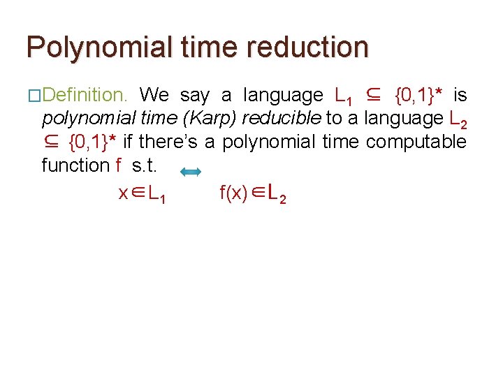
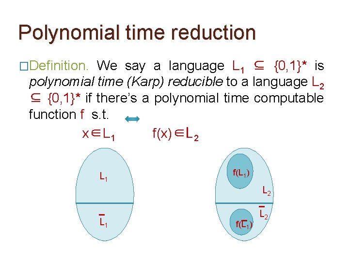
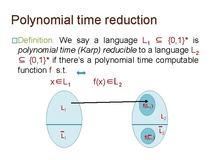
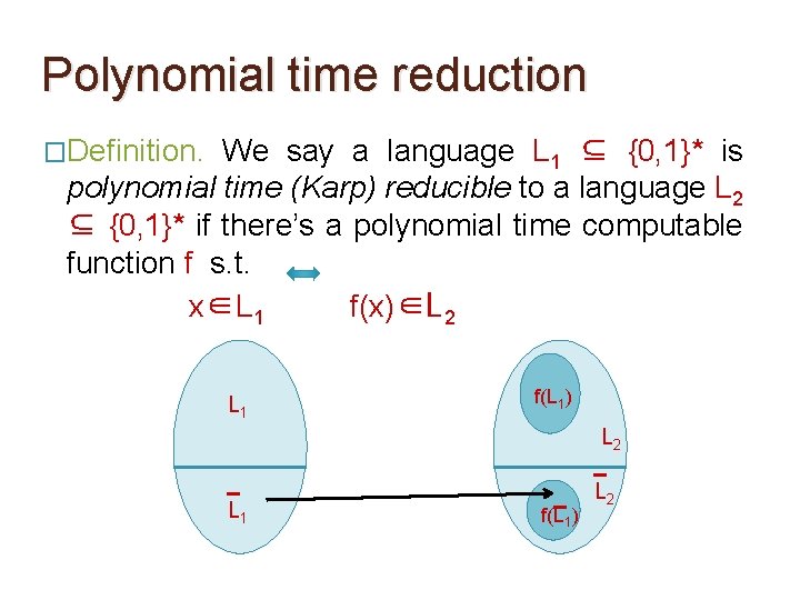
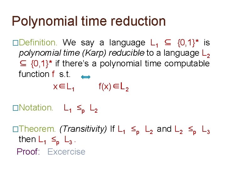
Polynomial time reduction �Definition. We say a language L 1 ⊆ {0, 1}* is polynomial time (Karp) reducible to a language L 2 ⊆ {0, 1}* if there’s a polynomial time computable function f s. t. x∈L 1 f(x)∈L 2
Polynomial time reduction �Definition. We say a language L 1 ⊆ {0, 1}* is polynomial time (Karp) reducible to a language L 2 ⊆ {0, 1}* if there’s a polynomial time computable function f s. t. x∈L 1 f(x)∈L 2 L 1 f(L 1) L 2
Polynomial time reduction �Definition. We say a language L 1 ⊆ {0, 1}* is polynomial time (Karp) reducible to a language L 2 ⊆ {0, 1}* if there’s a polynomial time computable function f s. t. x∈L 1 f(x)∈L 2 L 1 f(L 1) L 2
Polynomial time reduction �Definition. We say a language L 1 ⊆ {0, 1}* is polynomial time (Karp) reducible to a language L 2 ⊆ {0, 1}* if there’s a polynomial time computable function f s. t. x∈L 1 f(x)∈L 2 L 1 f(L 1) L 2
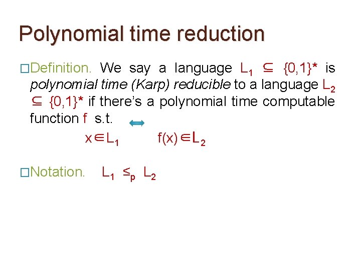
Polynomial time reduction �Definition. We say a language L 1 ⊆ {0, 1}* is polynomial time (Karp) reducible to a language L 2 ⊆ {0, 1}* if there’s a polynomial time computable function f s. t. x∈L 1 f(x)∈L 2 �Notation. L 1 ≤ p L 2
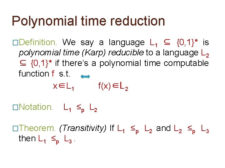
Polynomial time reduction �Definition. We say a language L 1 ⊆ {0, 1}* is polynomial time (Karp) reducible to a language L 2 ⊆ {0, 1}* if there’s a polynomial time computable function f s. t. x∈L 1 f(x)∈L 2 �Notation. �Theorem. L 1 ≤ p L 2 (Transitivity) If L 1 ≤p L 2 and L 2 ≤p L 3 then L 1 ≤p L 3.
Polynomial time reduction �Definition. We say a language L 1 ⊆ {0, 1}* is polynomial time (Karp) reducible to a language L 2 ⊆ {0, 1}* if there’s a polynomial time computable function f s. t. x∈L 1 f(x)∈L 2 �Notation. �Theorem. L 1 ≤ p L 2 (Transitivity) If L 1 ≤p L 2 and L 2 ≤p L 3 then L 1 ≤p L 3. Proof: Excercise
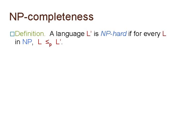
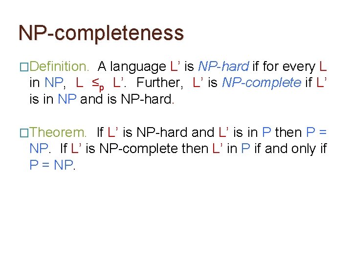
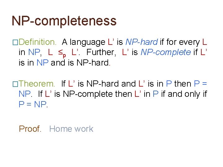
NP-completeness �Definition. A language L’ is NP-hard if for every L in NP, L ≤p L’.
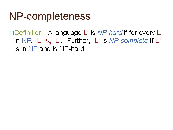
NP-completeness �Definition. A language L’ is NP-hard if for every L in NP, L ≤p L’. Further, L’ is NP-complete if L’ is in NP and is NP-hard.
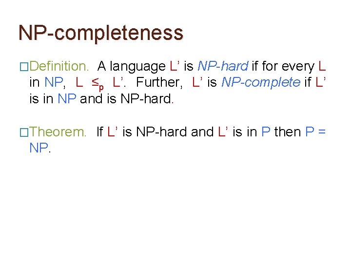
NP-completeness �Definition. A language L’ is NP-hard if for every L in NP, L ≤p L’. Further, L’ is NP-complete if L’ is in NP and is NP-hard. �Theorem. NP. If L’ is NP-hard and L’ is in P then P =
NP-completeness �Definition. A language L’ is NP-hard if for every L in NP, L ≤p L’. Further, L’ is NP-complete if L’ is in NP and is NP-hard. �Theorem. If L’ is NP-hard and L’ is in P then P = NP. If L’ is NP-complete then L’ in P if and only if P = NP.
NP-completeness �Definition. A language L’ is NP-hard if for every L in NP, L ≤p L’. Further, L’ is NP-complete if L’ is in NP and is NP-hard. �Theorem. If L’ is NP-hard and L’ is in P then P = NP. If L’ is NP-complete then L’ in P if and only if P = NP. Proof. Home work
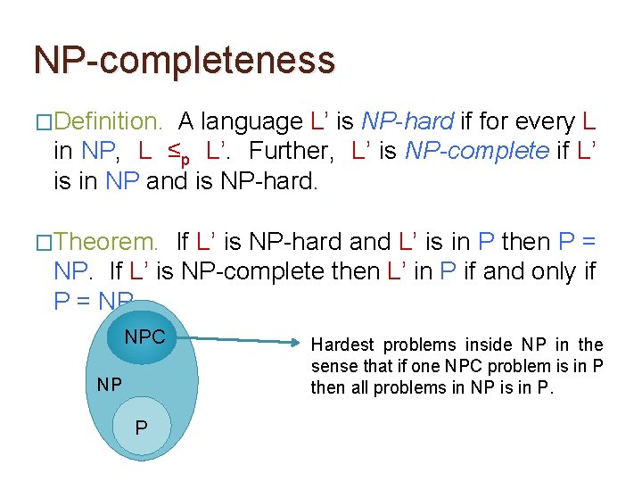
NP-completeness �Definition. A language L’ is NP-hard if for every L in NP, L ≤p L’. Further, L’ is NP-complete if L’ is in NP and is NP-hard. �Theorem. If L’ is NP-hard and L’ is in P then P = NP. If L’ is NP-complete then L’ in P if and only if P = NP. NPC NP P Hardest problems inside NP in the sense that if one NPC problem is in P then all problems in NP is in P.
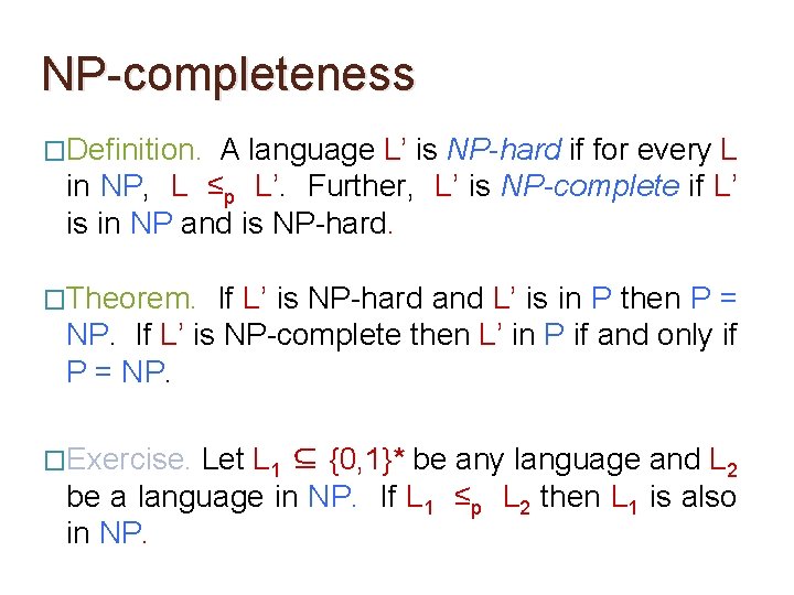
NP-completeness �Definition. A language L’ is NP-hard if for every L in NP, L ≤p L’. Further, L’ is NP-complete if L’ is in NP and is NP-hard. �Theorem. If L’ is NP-hard and L’ is in P then P = NP. If L’ is NP-complete then L’ in P if and only if P = NP. �Exercise. Let L 1 ⊆ {0, 1}* be any language and L 2 be a language in NP. If L 1 ≤p L 2 then L 1 is also in NP.
A few words on reductions �As to how we define a reduction from one language to the other (or one function to the other) is usually guided by a question on whether two complexity classes are different or identical.
A few words on reductions �As to how we define a reduction from one language to the other (or one function to the other) is usually guided by a question on whether two complexity classes are different or identical. �For polynomial time reductions, the question is whether P equals NP.
A few words on reductions �As to how we define a reduction from one language to the other (or one function to the other) is usually guided by a question on whether two complexity classes are different or identical. �For polynomial time reductions, the question is whether P equals NP. �Reductions help us define complete problems (the ‘hardest’ problems in a class) which in turn help us compare the complexity classes under consideration.
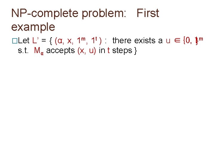
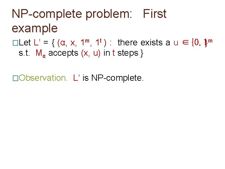
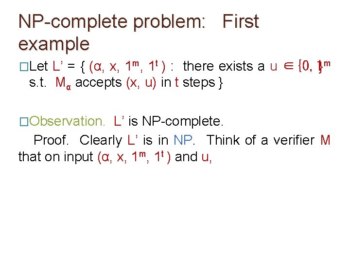
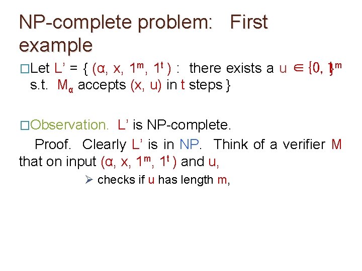
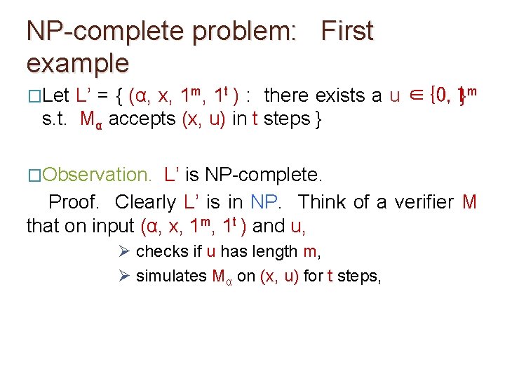
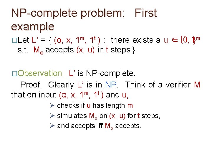
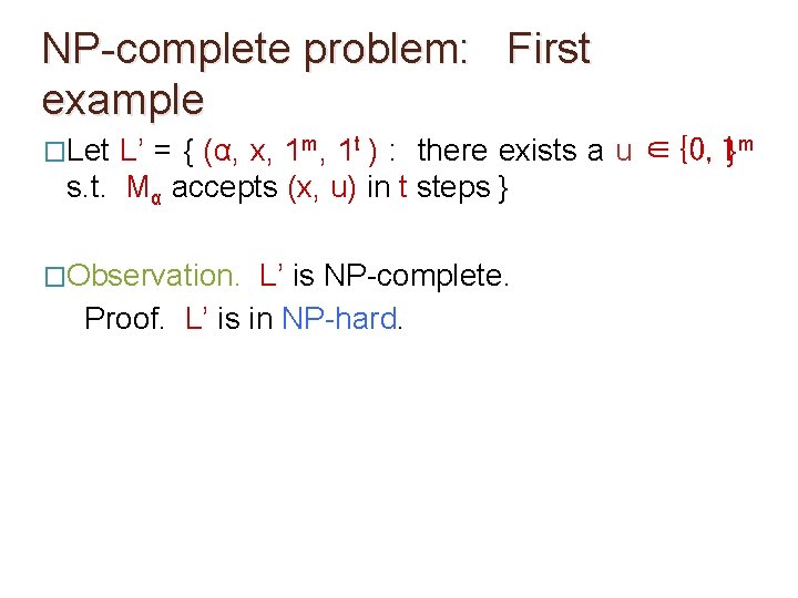
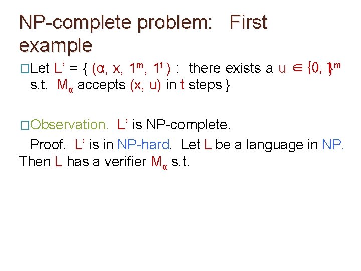
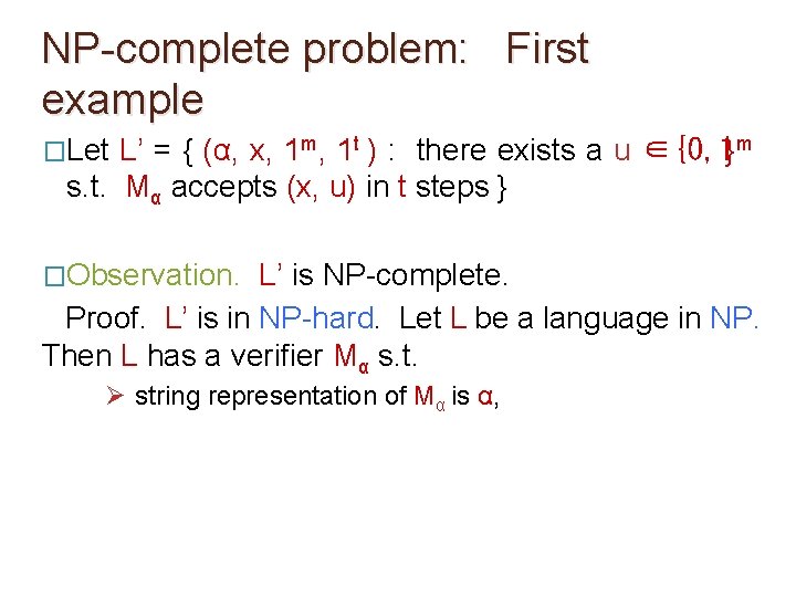
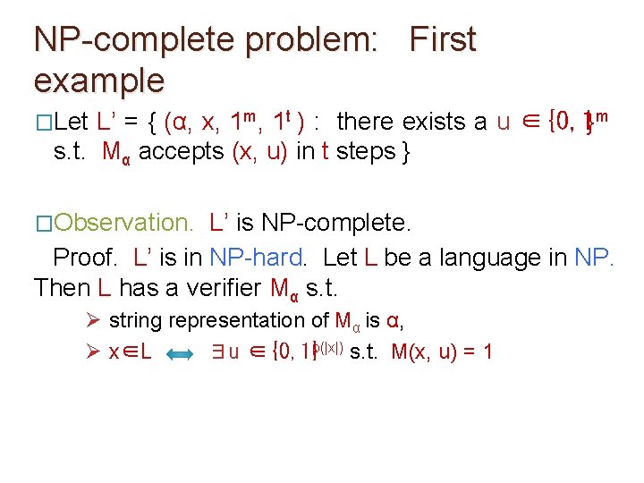
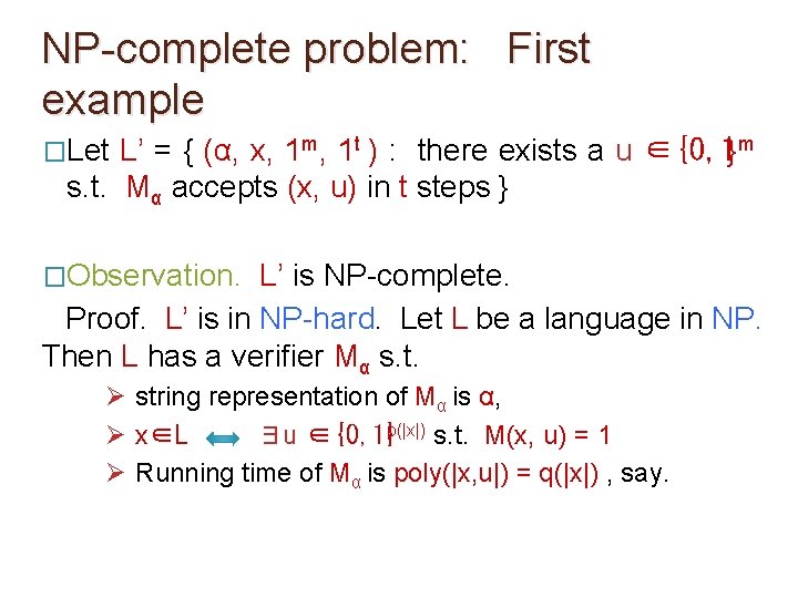
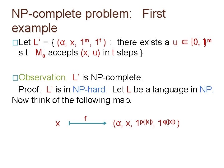
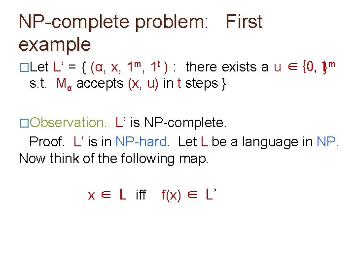
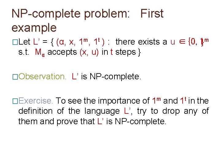
NP-complete problem: First example �Let L’ = { (α, x, 1 m, 1 t ) : there exists a u ∈{0, 1}m s. t. Mα accepts (x, u) in t steps }
NP-complete problem: First example �Let L’ = { (α, x, 1 m, 1 t ) : there exists a u ∈{0, 1}m s. t. Mα accepts (x, u) in t steps } �Observation. L’ is NP-complete.
NP-complete problem: First example �Let L’ = { (α, x, 1 m, 1 t ) : there exists a u ∈{0, 1}m s. t. Mα accepts (x, u) in t steps } �Observation. L’ is NP-complete. Proof. Clearly L’ is in NP. Think of a verifier M that on input (α, x, 1 m, 1 t ) and u,
NP-complete problem: First example �Let L’ = { (α, x, 1 m, 1 t ) : there exists a u ∈{0, 1}m s. t. Mα accepts (x, u) in t steps } �Observation. L’ is NP-complete. Proof. Clearly L’ is in NP. Think of a verifier M that on input (α, x, 1 m, 1 t ) and u, Ø checks if u has length m,
NP-complete problem: First example �Let L’ = { (α, x, 1 m, 1 t ) : there exists a u ∈{0, 1}m s. t. Mα accepts (x, u) in t steps } �Observation. L’ is NP-complete. Proof. Clearly L’ is in NP. Think of a verifier M that on input (α, x, 1 m, 1 t ) and u, Ø checks if u has length m, Ø simulates Mα on (x, u) for t steps,
NP-complete problem: First example �Let L’ = { (α, x, 1 m, 1 t ) : there exists a u ∈{0, 1}m s. t. Mα accepts (x, u) in t steps } �Observation. L’ is NP-complete. Proof. Clearly L’ is in NP. Think of a verifier M that on input (α, x, 1 m, 1 t ) and u, Ø checks if u has length m, Ø simulates Mα on (x, u) for t steps, Ø and accepts iff Mα accepts.
NP-complete problem: First example �Let L’ = { (α, x, 1 m, 1 t ) : there exists a u ∈{0, 1}m s. t. Mα accepts (x, u) in t steps } �Observation. L’ is NP-complete. Proof. L’ is in NP-hard.
NP-complete problem: First example �Let L’ = { (α, x, 1 m, 1 t ) : there exists a u ∈{0, 1}m s. t. Mα accepts (x, u) in t steps } �Observation. L’ is NP-complete. Proof. L’ is in NP-hard. Let L be a language in NP. Then L has a verifier Mα s. t.
NP-complete problem: First example �Let L’ = { (α, x, 1 m, 1 t ) : there exists a u ∈{0, 1}m s. t. Mα accepts (x, u) in t steps } �Observation. L’ is NP-complete. Proof. L’ is in NP-hard. Let L be a language in NP. Then L has a verifier Mα s. t. Ø string representation of Mα is α,
NP-complete problem: First example �Let L’ = { (α, x, 1 m, 1 t ) : there exists a u ∈{0, 1}m s. t. Mα accepts (x, u) in t steps } �Observation. L’ is NP-complete. Proof. L’ is in NP-hard. Let L be a language in NP. Then L has a verifier Mα s. t. Ø string representation of Mα is α, Ø x∈L ∃u ∈{0, 1}p(|x|) s. t. M(x, u) = 1
NP-complete problem: First example �Let L’ = { (α, x, 1 m, 1 t ) : there exists a u ∈{0, 1}m s. t. Mα accepts (x, u) in t steps } �Observation. L’ is NP-complete. Proof. L’ is in NP-hard. Let L be a language in NP. Then L has a verifier Mα s. t. Ø string representation of Mα is α, Ø x∈L ∃u ∈{0, 1}p(|x|) s. t. M(x, u) = 1 Ø Running time of Mα is poly(|x, u|) = q(|x|) , say.
NP-complete problem: First example �Let L’ = { (α, x, 1 m, 1 t ) : there exists a u ∈{0, 1}m s. t. Mα accepts (x, u) in t steps } �Observation. L’ is NP-complete. Proof. L’ is in NP-hard. Let L be a language in NP. Now think of the following map. x f (α, x, 1 p(|x|), 1 q(|x|) )
NP-complete problem: First example �Let L’ = { (α, x, 1 m, 1 t ) : there exists a u ∈{0, 1}m s. t. Mα accepts (x, u) in t steps } �Observation. L’ is NP-complete. Proof. L’ is in NP-hard. Let L be a language in NP. Now think of the following map. x ∈ L iff f(x) ∈ L’
NP-complete problem: First example �Let L’ = { (α, x, 1 m, 1 t ) : there exists a u ∈{0, 1}m s. t. Mα accepts (x, u) in t steps } �Observation. �Exercise. L’ is NP-complete. To see the importance of 1 m and 1 t in the definition of the language L’, try to drop any of them and prove that L’ is NP-complete.
A natural NP-complete problem �The language L’ involves Turing machine in its definition. Next, we’ll see an example of an NPcomplete problem that is arguably more natural.
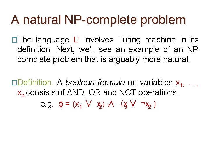
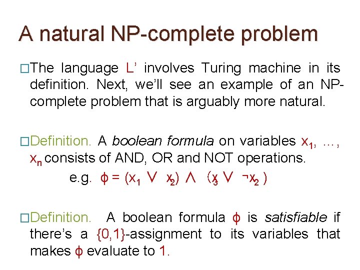
A natural NP-complete problem �The language L’ involves Turing machine in its definition. Next, we’ll see an example of an NPcomplete problem that is arguably more natural. �Definition. A boolean formula on variables x 1, …, xn consists of AND, OR and NOT operations. e. g. ϕ = (x 1 ∨ x 2) ∧ (x 3 ∨ ¬x 2 )
A natural NP-complete problem �The language L’ involves Turing machine in its definition. Next, we’ll see an example of an NPcomplete problem that is arguably more natural. �Definition. A boolean formula on variables x 1, …, xn consists of AND, OR and NOT operations. e. g. ϕ = (x 1 ∨ x 2) ∧ (x 3 ∨ ¬x 2 ) �Definition. A boolean formula ϕ is satisfiable if there’s a {0, 1}-assignment to its variables that makes ϕ evaluate to 1.
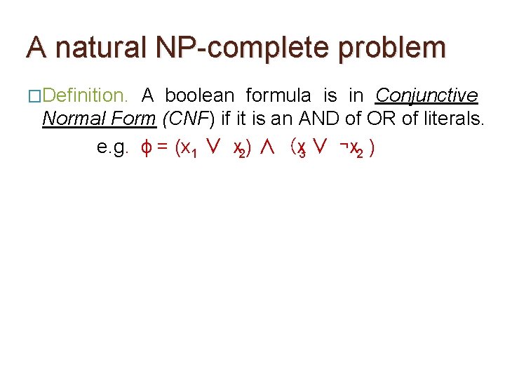
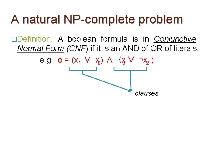
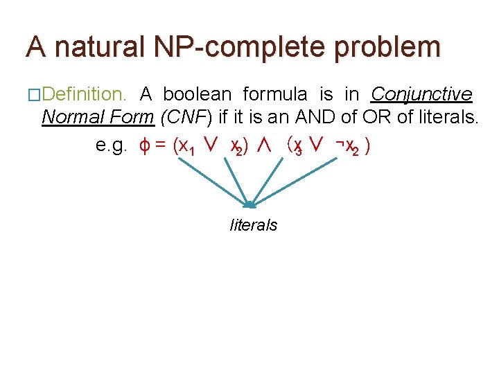
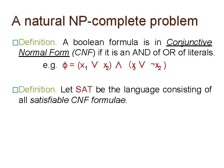
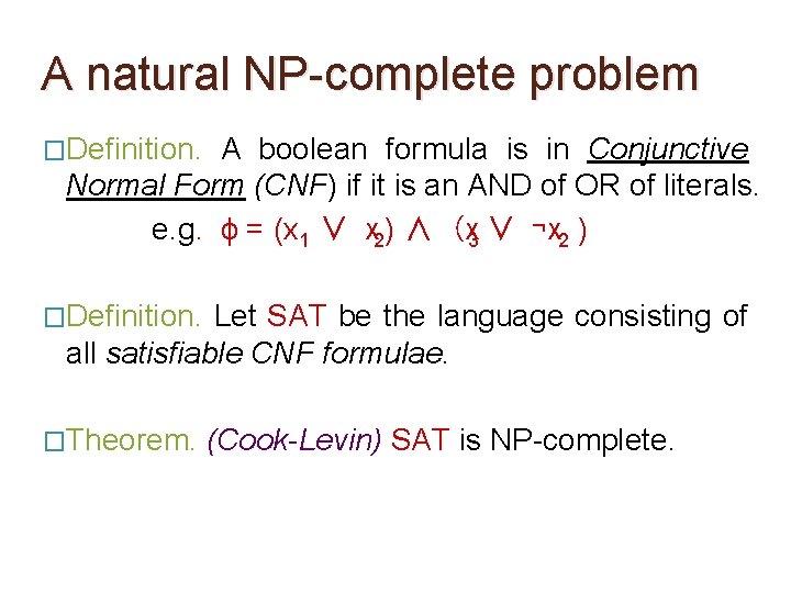
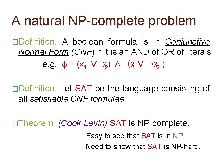
A natural NP-complete problem �Definition. A boolean formula is in Conjunctive Normal Form (CNF) if it is an AND of OR of literals. e. g. ϕ = (x 1 ∨ x 2) ∧ (x 3 ∨ ¬x 2 )
A natural NP-complete problem �Definition. A boolean formula is in Conjunctive Normal Form (CNF) if it is an AND of OR of literals. e. g. ϕ = (x 1 ∨ x 2) ∧ (x 3 ∨ ¬x 2 ) clauses
A natural NP-complete problem �Definition. A boolean formula is in Conjunctive Normal Form (CNF) if it is an AND of OR of literals. e. g. ϕ = (x 1 ∨ x 2) ∧ (x 3 ∨ ¬x 2 ) literals
A natural NP-complete problem �Definition. A boolean formula is in Conjunctive Normal Form (CNF) if it is an AND of OR of literals. e. g. ϕ = (x 1 ∨ x 2) ∧ (x 3 ∨ ¬x 2 ) �Definition. Let SAT be the language consisting of all satisfiable CNF formulae.
A natural NP-complete problem �Definition. A boolean formula is in Conjunctive Normal Form (CNF) if it is an AND of OR of literals. e. g. ϕ = (x 1 ∨ x 2) ∧ (x 3 ∨ ¬x 2 ) �Definition. Let SAT be the language consisting of all satisfiable CNF formulae. �Theorem. (Cook-Levin) SAT is NP-complete.
A natural NP-complete problem �Definition. A boolean formula is in Conjunctive Normal Form (CNF) if it is an AND of OR of literals. e. g. ϕ = (x 1 ∨ x 2) ∧ (x 3 ∨ ¬x 2 ) �Definition. Let SAT be the language consisting of all satisfiable CNF formulae. �Theorem. (Cook-Levin) SAT is NP-complete. Easy to see that SAT is in NP. Need to show that SAT is NP-hard.
Cook-Levin theorem: Proof �Main idea: Computation is local;
Cook-Levin theorem: Proof �Main idea: Computation is local; i. e. every step of computation looks at and changes only constantly many bits;
Cook-Levin theorem: Proof �Main idea: Computation is local; i. e. every step of computation looks at and changes only constantly many bits; and hence this step can be implemented by a small CNF formula.
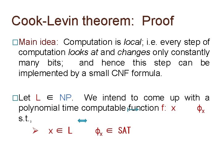
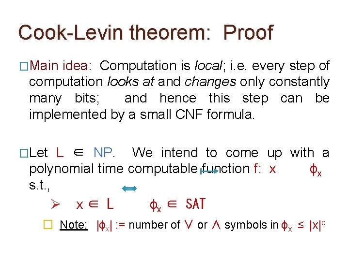
Cook-Levin theorem: Proof �Main idea: Computation is local; i. e. every step of computation looks at and changes only constantly many bits; and hence this step can be implemented by a small CNF formula. �Let L ∈ NP. We intend to come up with a polynomial time computable function f: x ϕx s. t. , Ø x∈ L ϕx ∈ SAT
Cook-Levin theorem: Proof �Main idea: Computation is local; i. e. every step of computation looks at and changes only constantly many bits; and hence this step can be implemented by a small CNF formula. �Let L ∈ NP. We intend to come up with a polynomial time computable function f: x ϕx s. t. , Ø x∈ L ϕx ∈ SAT � Note: |ϕx| : = number of ∨ or ∧ symbols in ϕx ≤ |x|c
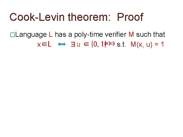
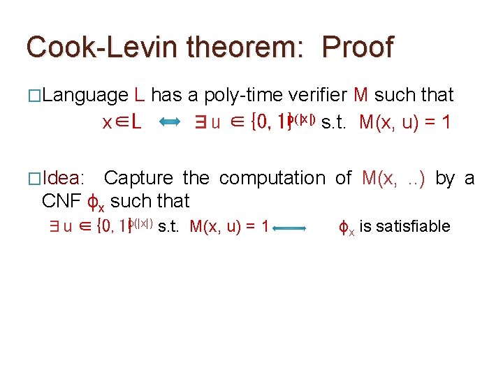
Cook-Levin theorem: Proof �Language L has a poly-time verifier M such that x∈L ∃u ∈{0, 1}p(|x|) s. t. M(x, u) = 1
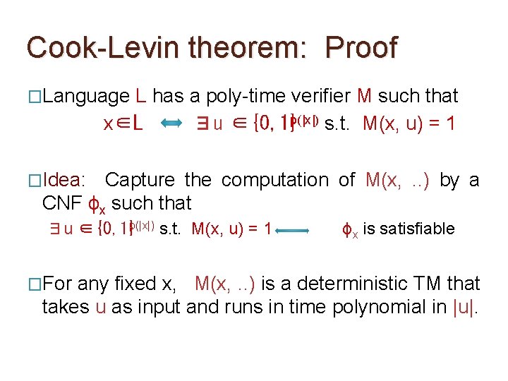
Cook-Levin theorem: Proof �Language L has a poly-time verifier M such that x∈L ∃u ∈{0, 1}p(|x|) s. t. M(x, u) = 1 �Idea: Capture the computation of M(x, . . ) by a CNF ϕx such that ∃u ∈{0, 1}p(|x|) s. t. M(x, u) = 1 ϕx is satisfiable
Cook-Levin theorem: Proof �Language L has a poly-time verifier M such that x∈L ∃u ∈{0, 1}p(|x|) s. t. M(x, u) = 1 �Idea: Capture the computation of M(x, . . ) by a CNF ϕx such that ∃u ∈{0, 1}p(|x|) s. t. M(x, u) = 1 �For ϕx is satisfiable any fixed x, M(x, . . ) is a deterministic TM that takes u as input and runs in time polynomial in |u|.
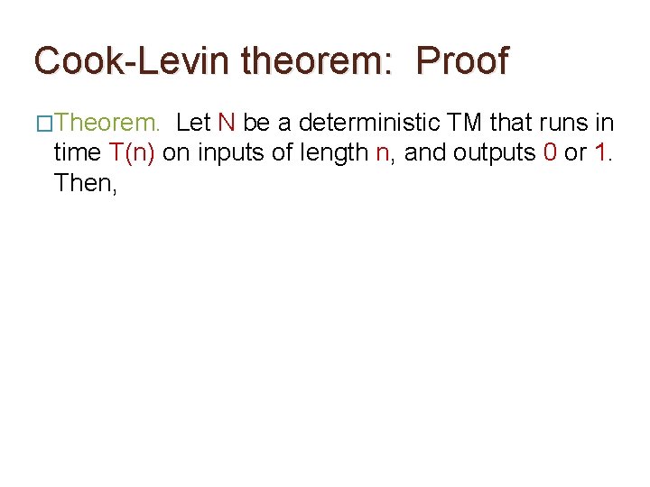
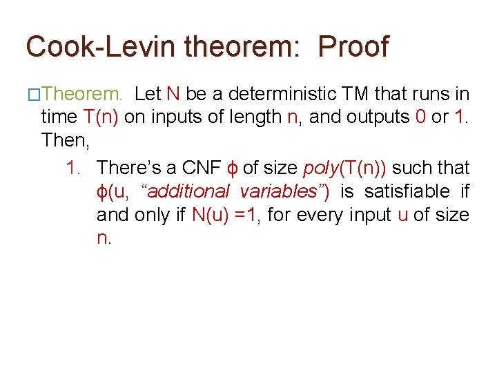
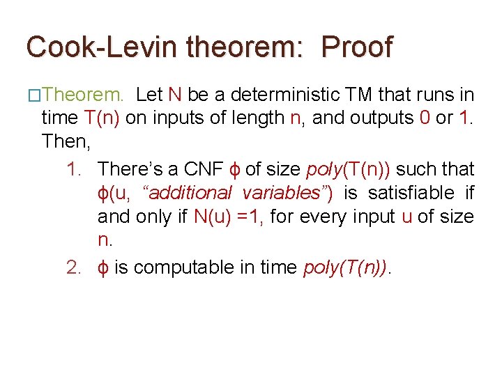
Cook-Levin theorem: Proof �Theorem. Let N be a deterministic TM that runs in time T(n) on inputs of length n, and outputs 0 or 1. Then,
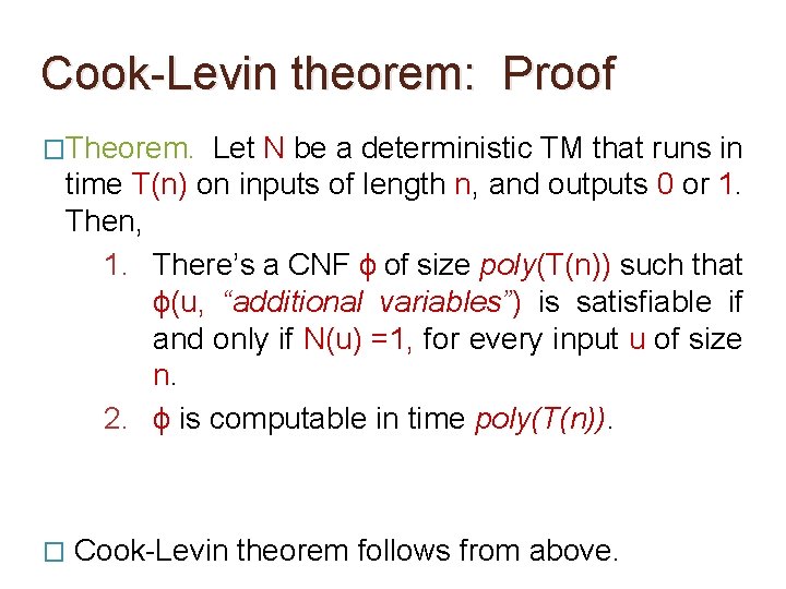
Cook-Levin theorem: Proof �Theorem. Let N be a deterministic TM that runs in time T(n) on inputs of length n, and outputs 0 or 1. Then, 1. There’s a CNF ϕ of size poly(T(n)) such that ϕ(u, “additional variables”) is satisfiable if and only if N(u) =1, for every input u of size n.
Cook-Levin theorem: Proof �Theorem. Let N be a deterministic TM that runs in time T(n) on inputs of length n, and outputs 0 or 1. Then, 1. There’s a CNF ϕ of size poly(T(n)) such that ϕ(u, “additional variables”) is satisfiable if and only if N(u) =1, for every input u of size n. 2. ϕ is computable in time poly(T(n)).
Cook-Levin theorem: Proof �Theorem. Let N be a deterministic TM that runs in time T(n) on inputs of length n, and outputs 0 or 1. Then, 1. There’s a CNF ϕ of size poly(T(n)) such that ϕ(u, “additional variables”) is satisfiable if and only if N(u) =1, for every input u of size n. 2. ϕ is computable in time poly(T(n)). � Cook-Levin theorem follows from above.
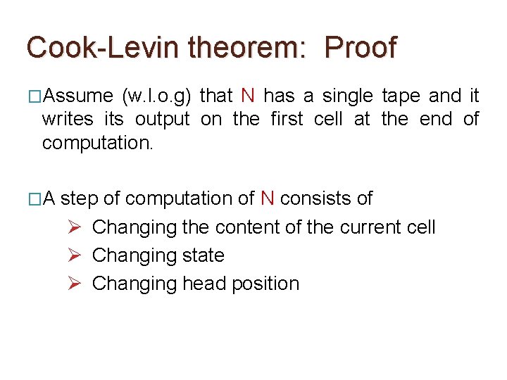
Cook-Levin theorem: Proof �Assume (w. l. o. g) that N has a single tape and it writes its output on the first cell at the end of computation.
Cook-Levin theorem: Proof �Assume (w. l. o. g) that N has a single tape and it writes its output on the first cell at the end of computation. �A step of computation of N consists of Ø Changing the content of the current cell Ø Changing state Ø Changing head position
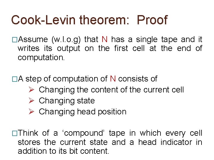
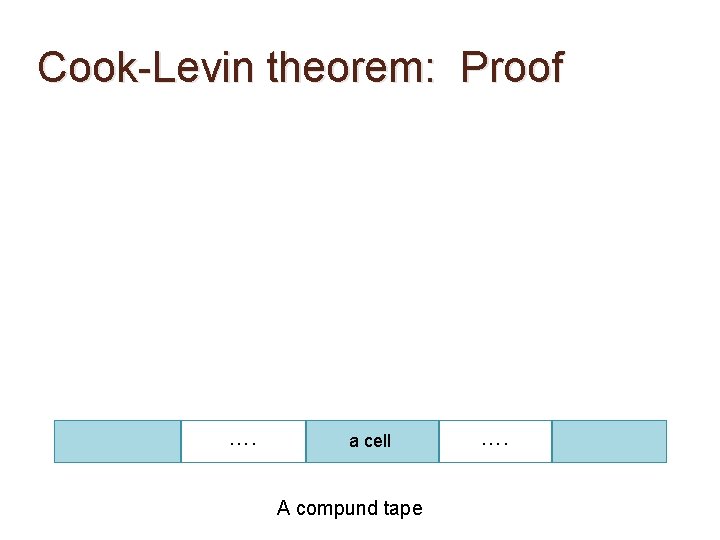
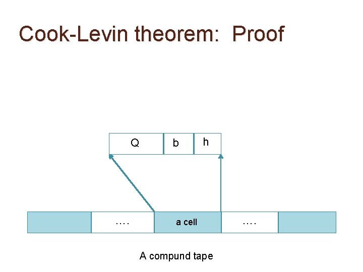
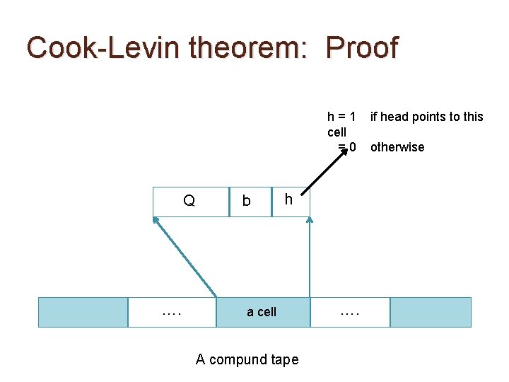
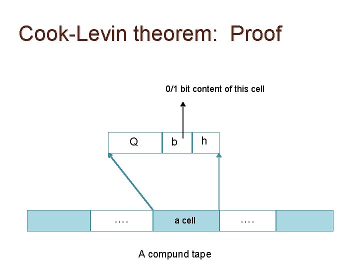
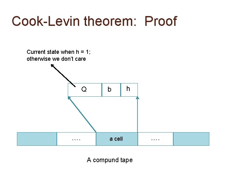
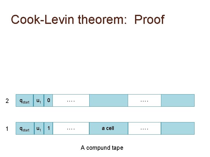
Cook-Levin theorem: Proof �Assume (w. l. o. g) that N has a single tape and it writes its output on the first cell at the end of computation. �A step of computation of N consists of Ø Changing the content of the current cell Ø Changing state Ø Changing head position �Think of a ‘compound’ tape in which every cell stores the current state and a head indicator in addition to its bit content.
Cook-Levin theorem: Proof …. a cell A compund tape ….
Cook-Levin theorem: Proof Q …. b h a cell A compund tape ….
Cook-Levin theorem: Proof h=1 cell =0 Q …. b h a cell A compund tape …. if head points to this otherwise
Cook-Levin theorem: Proof 0/1 bit content of this cell Q …. b h a cell A compund tape ….
Cook-Levin theorem: Proof Current state when h = 1; otherwise we don’t care Q …. b h a cell A compund tape ….
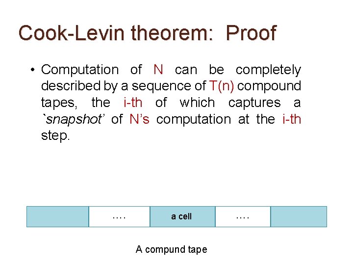
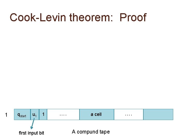
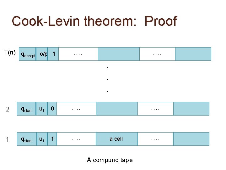
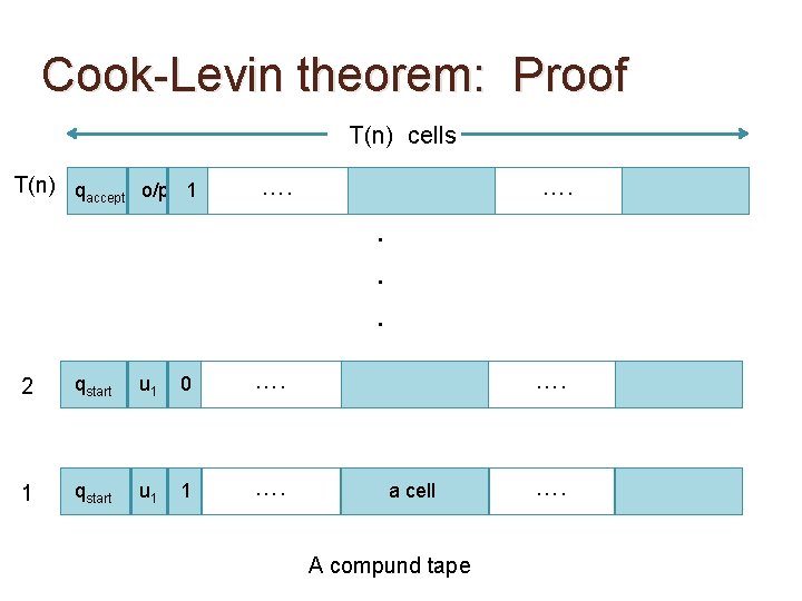
Cook-Levin theorem: Proof • Computation of N can be completely described by a sequence of T(n) compound tapes, the i-th of which captures a `snapshot’ of N’s computation at the i-th step. …. a cell A compund tape ….
Cook-Levin theorem: Proof 1 qstart u 1 1 first input bit …. a cell A compund tape ….
Cook-Levin theorem: Proof 2 qstart u 1 0 …. 1 qstart u 1 1 …. a cell A compund tape ….
Cook-Levin theorem: Proof T(n) qaccept o/p 1 …. . . . 2 qstart u 1 0 …. 1 qstart u 1 1 …. a cell A compund tape ….
Cook-Levin theorem: Proof T(n) cells T(n) qaccept o/p 1 …. . . . 2 qstart u 1 0 …. 1 qstart u 1 1 …. a cell A compund tape ….
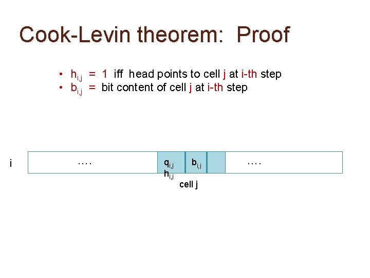
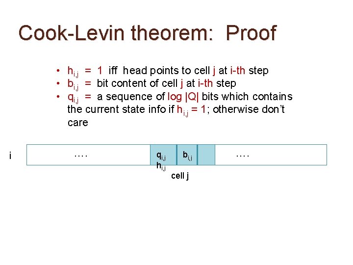
Cook-Levin theorem: Proof • hi, j = 1 iff head points to cell j at i-th step • bi, j = bit content of cell j at i-th step i …. qi, j hi, j bi, j cell j ….
Cook-Levin theorem: Proof • hi, j = 1 iff head points to cell j at i-th step • bi, j = bit content of cell j at i-th step • qi, j = a sequence of log |Q| bits which contains the current state info if hi, j = 1; otherwise don’t care i …. qi, j hi, j bi, j cell j ….
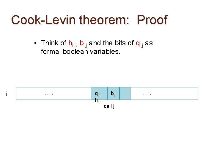
Cook-Levin theorem: Proof • Think of hi, j, bi, j and the bits of qi, j as formal boolean variables. i …. qi, j hi, j bi, j cell j ….
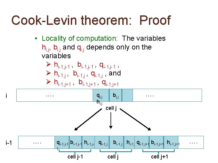
Cook-Levin theorem: Proof • Locality of computation: The variables hi, j, bi, j and qi, j depends only on the variables Ø hi-1, j-1 , bi-1, j-1 , qi-1, j-1 , Ø hi-1, j , bi-1, j , qi-1, j , and Ø hi-1, j+1 , bi-1, j+1 , qi-1, j+1 …. i i-1 …. qi, j hi, j bi, j …. cell j qi-1, j-1 bi-1, j-1 hi-1, j- qi-1, j bi-1, j hi-1, j qi-1, j+1 bi-1, j+1 hi-1, j+1 1 cell j-1 cell j+1 ….
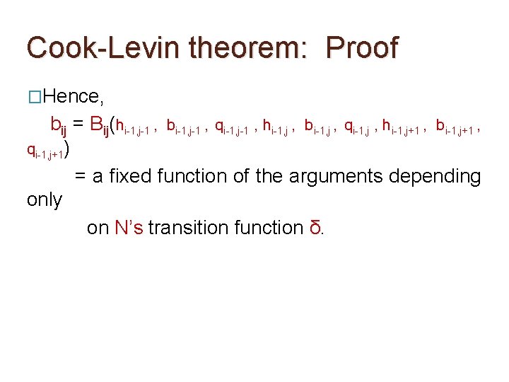
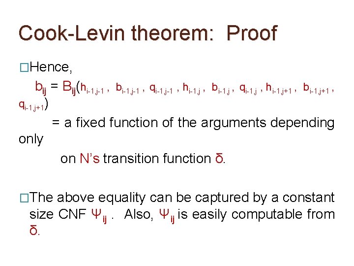
Cook-Levin theorem: Proof �Hence, bij = Bij(hi-1, j-1 , bi-1, j-1 , qi-1, j-1 , hi-1, j , bi-1, j , qi-1, j , hi-1, j+1 , bi-1, j+1 , qi-1, j+1) = a fixed function of the arguments depending only on N’s transition function δ.
Cook-Levin theorem: Proof �Hence, bij = Bij(hi-1, j-1 , bi-1, j-1 , qi-1, j-1 , hi-1, j , bi-1, j , qi-1, j , hi-1, j+1 , bi-1, j+1 , qi-1, j+1) = a fixed function of the arguments depending only on N’s transition function δ. �The above equality can be captured by a constant size CNF Ψij. Also, Ψij is easily computable from δ.
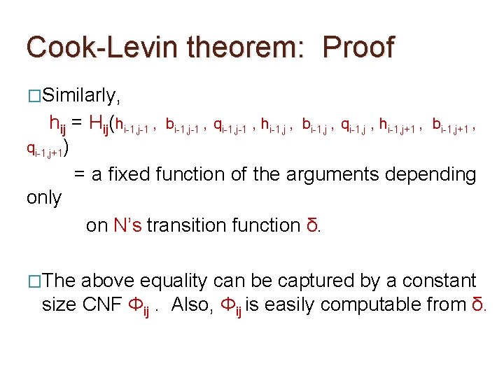
Cook-Levin theorem: Proof �Similarly, hij = Hij(hi-1, j-1 , bi-1, j-1 , qi-1, j-1 , hi-1, j , bi-1, j , qi-1, j , hi-1, j+1 , bi-1, j+1 , qi-1, j+1) = a fixed function of the arguments depending only on N’s transition function δ. �The above equality can be captured by a constant size CNF Φij. Also, Φij is easily computable from δ.
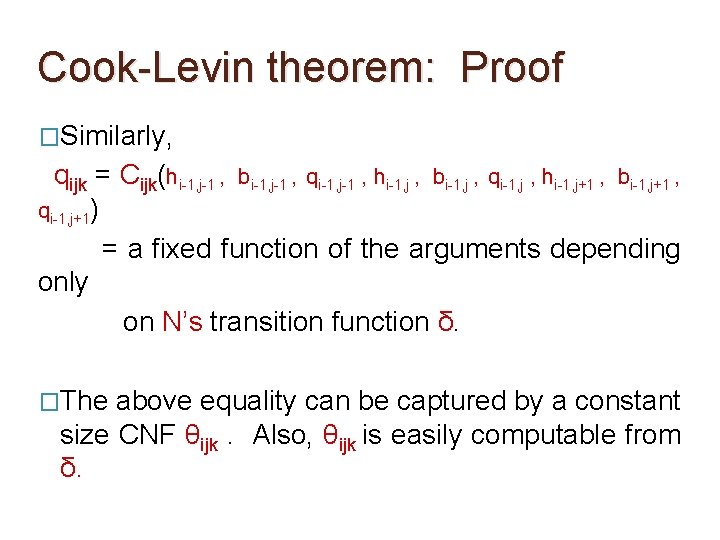
Cook-Levin theorem: Proof �Similarly, qijk = Cijk(hi-1, j-1 , bi-1, j-1 , qi-1, j-1 , hi-1, j , bi-1, j , qi-1, j , hi-1, j+1 , bi-1, j+1 , qi-1, j+1) = a fixed function of the arguments depending only on N’s transition function δ. �The above equality can be captured by a constant size CNF θijk. Also, θijk is easily computable from δ.
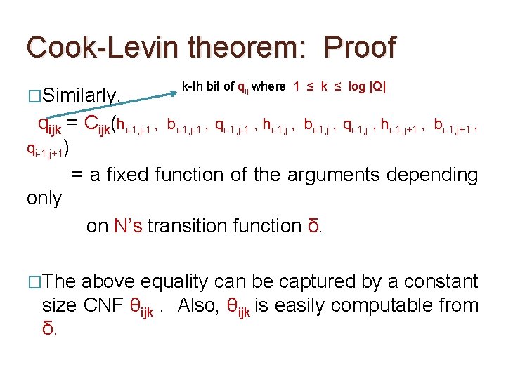
Cook-Levin theorem: Proof �Similarly, k-th bit of qij where 1 ≤ k ≤ log |Q| qijk = Cijk(hi-1, j-1 , bi-1, j-1 , qi-1, j-1 , hi-1, j , bi-1, j , qi-1, j , hi-1, j+1 , bi-1, j+1 , qi-1, j+1) = a fixed function of the arguments depending only on N’s transition function δ. �The above equality can be captured by a constant size CNF θijk. Also, θijk is easily computable from δ.
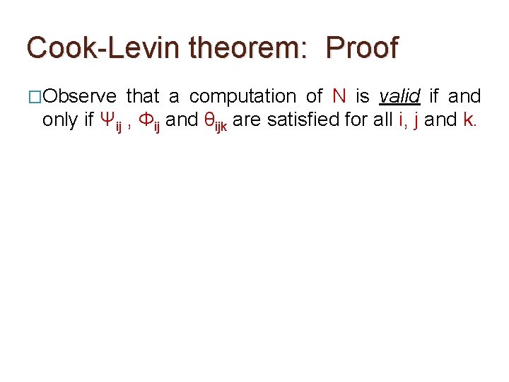
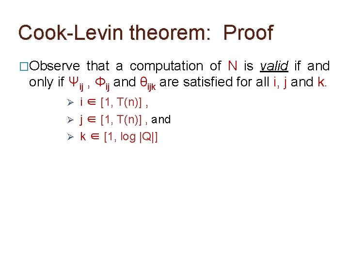
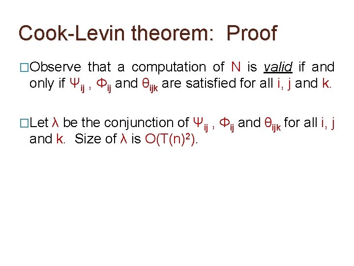
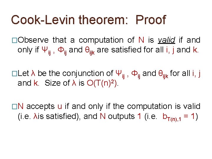
Cook-Levin theorem: Proof �Observe that a computation of N is valid if and only if Ψij , Φij and θijk are satisfied for all i, j and k.
Cook-Levin theorem: Proof �Observe that a computation of N is valid if and only if Ψij , Φij and θijk are satisfied for all i, j and k. Ø i ∈ [1, T(n)] , j ∈ [1, T(n)] , and Ø k ∈ [1, log |Q|] Ø
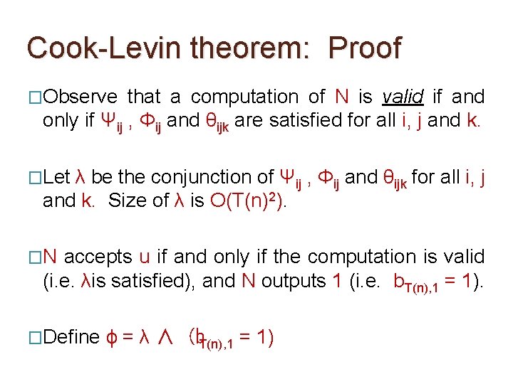
Cook-Levin theorem: Proof �Observe that a computation of N is valid if and only if Ψij , Φij and θijk are satisfied for all i, j and k. �Let λ be the conjunction of Ψij , Φij and θijk for all i, j and k. Size of λ is O(T(n)2).
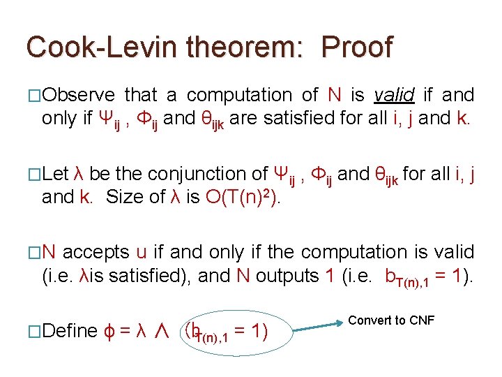
Cook-Levin theorem: Proof �Observe that a computation of N is valid if and only if Ψij , Φij and θijk are satisfied for all i, j and k. �Let λ be the conjunction of Ψij , Φij and θijk for all i, j and k. Size of λ is O(T(n)2). �N accepts u if and only if the computation is valid (i. e. λis satisfied), and N outputs 1 (i. e. b. T(n), 1 = 1)
Cook-Levin theorem: Proof �Observe that a computation of N is valid if and only if Ψij , Φij and θijk are satisfied for all i, j and k. �Let λ be the conjunction of Ψij , Φij and θijk for all i, j and k. Size of λ is O(T(n)2). �N accepts u if and only if the computation is valid (i. e. λis satisfied), and N outputs 1 (i. e. b. T(n), 1 = 1). �Define ϕ = λ ∧ (b. T(n), 1 = 1)
Cook-Levin theorem: Proof �Observe that a computation of N is valid if and only if Ψij , Φij and θijk are satisfied for all i, j and k. �Let λ be the conjunction of Ψij , Φij and θijk for all i, j and k. Size of λ is O(T(n)2). �N accepts u if and only if the computation is valid (i. e. λis satisfied), and N outputs 1 (i. e. b. T(n), 1 = 1). �Define ϕ = λ ∧ (b. T(n), 1 = 1) Convert to CNF
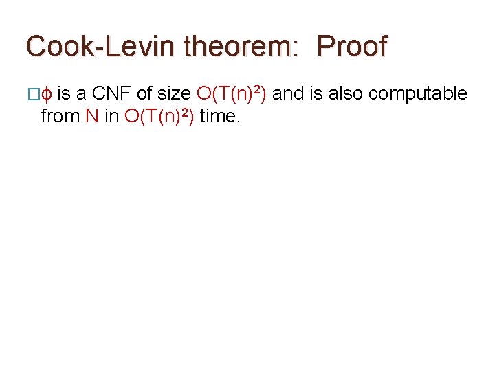
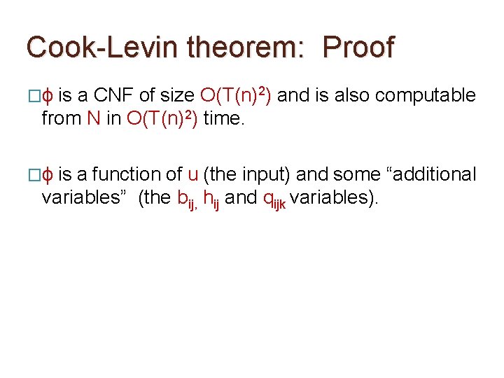
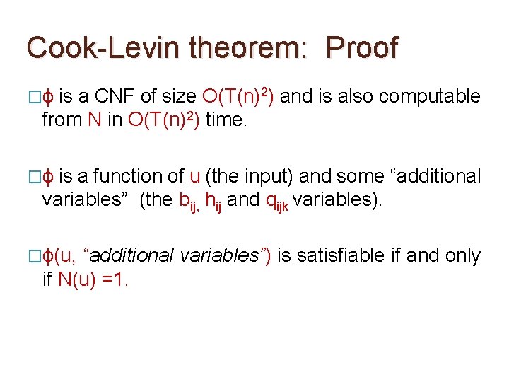
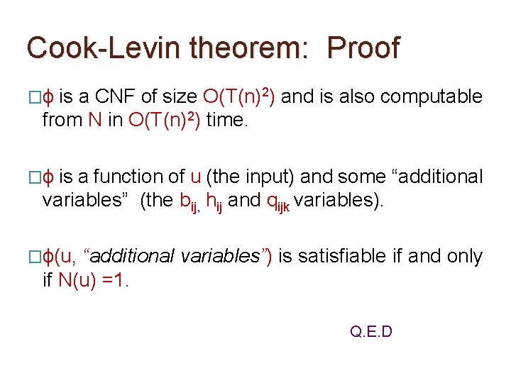
Cook-Levin theorem: Proof �ϕ is a CNF of size O(T(n)2) and is also computable from N in O(T(n)2) time.
Cook-Levin theorem: Proof �ϕ is a CNF of size O(T(n)2) and is also computable from N in O(T(n)2) time. �ϕ is a function of u (the input) and some “additional variables” (the bij, hij and qijk variables).
Cook-Levin theorem: Proof �ϕ is a CNF of size O(T(n)2) and is also computable from N in O(T(n)2) time. �ϕ is a function of u (the input) and some “additional variables” (the bij, hij and qijk variables). �ϕ(u, “additional variables”) is satisfiable if and only if N(u) =1.
Cook-Levin theorem: Proof �ϕ is a CNF of size O(T(n)2) and is also computable from N in O(T(n)2) time. �ϕ is a function of u (the input) and some “additional variables” (the bij, hij and qijk variables). �ϕ(u, “additional variables”) is satisfiable if and only if N(u) =1. Q. E. D
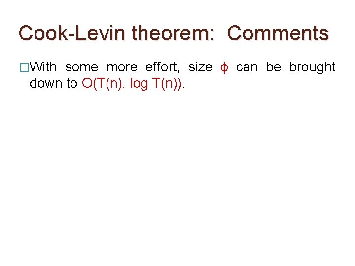
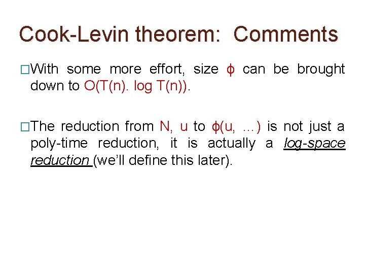
Cook-Levin theorem: Comments �With some more effort, size ϕ can be brought down to O(T(n). log T(n)).
Cook-Levin theorem: Comments �With some more effort, size ϕ can be brought down to O(T(n). log T(n)). �The reduction from N, u to ϕ(u, …) is not just a poly-time reduction, it is actually a log-space reduction (we’ll define this later).
Cook-Levin theorem: Comments �With some more effort, size ϕ can be brought down to O(T(n). log T(n)). �The reduction from N, u to ϕ(u, …) is not just a poly-time reduction, it is actually a log-space reduction (we’ll define this later). �Observe that once u is fixed the values of the “additional variables” are also determined
Cook-Levin theorem: Comments �With some more effort, size ϕ can be brought down to O(T(n). log T(n)). �The reduction from N, u to ϕ(u, …) is not just a poly-time reduction, it is actually a log-space reduction (we’ll define this later). �Observe that once u is fixed the values of the “additional variables” are also determined (in polynomial time).
Cook-Levin theorem: Comments �With some more effort, size ϕ can be brought down to O(T(n). log T(n)). �The reduction from N, u to ϕ(u, …) is not just a poly-time reduction, it is actually a log-space reduction (we’ll define this later). �Each clause of literals. ϕ has only constantly many