Matters of Time Space Today Time Space Complexity
![Size • Number of inputs processed • n int sum. Int. Array(int arr[ ], Size • Number of inputs processed • n int sum. Int. Array(int arr[ ],](https://slidetodoc.com/presentation_image_h/18769c89dbe3eb15931a425b90b51432/image-8.jpg)
- Slides: 26

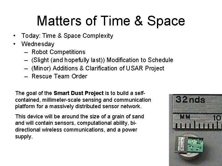
Matters of Time & Space • Today: Time & Space Complexity • Wednesday – Robot Competitions – (Slight (and hopefully last)) Modification to Schedule – (Minor) Additions & Clarification of USAR Project – Rescue Team Order The goal of the Smart Dust Project is to build a selfcontained, millimeter-scale sensing and communication platform for a massively distributed sensor network. This device will be around the size of a grain of sand will contain sensors, computational ability, bidirectional wireless communications, and a power supply.

Computational Resources • Time – How much time does it take for the program to run on a particular problem? • Space – How much memory space does it take for the program to run on a particular problem? • Processors are getting faster and memory is getting cheaper so why worry? – Limited resources in embedded computing like cars, cell phones, sensor networks, and robots – Real-time constraints

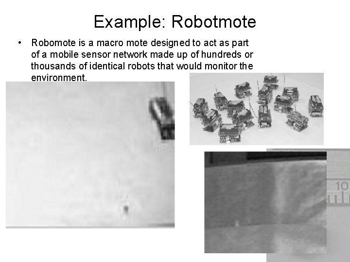
Example: Robotmote • Robomote is a macro mote designed to act as part of a mobile sensor network made up of hundreds or thousands of identical robots that would monitor the environment.

How do you compare programs? • Benchmarking – A standard program or set of programs which can be run on different computers to give an inaccurate measure of their performance. – http: //netlib. org/benchweb/ – "In the computer industry, there are three kinds of lies: lies, damn lies, and benchmarks. " • Why?

Algorithm Analysis • Compare running times and space requirements independent of programming languages, compiler, hardware, processor speed, … • Algorithm Analysis – Measure the efficiency of an algorithm or program as the size of the input becomes large – Provides a gross comparison of algorithms

Time & Space Complexity • Time Complexity – The way in which the number of steps required by a algorithm varies with the size of the problem it is solving. • Space Complexity – The way in which the amount of storage space required by an algorithm varies with the size of the problem it is solving. • What is meant by “steps” and “size”?

Steps • Basic operation – An algorithm step or program code that has the property that its time to complete does not depend on the particular values of its operands total. Error =total. Error + current. Error; for (i = 0; i < room. Length; i++) for (j = 0; j < room. Width; j++) { map(room[i, j]; … }
![Size Number of inputs processed n int sum Int Arrayint arr Size • Number of inputs processed • n int sum. Int. Array(int arr[ ],](https://slidetodoc.com/presentation_image_h/18769c89dbe3eb15931a425b90b51432/image-8.jpg)
Size • Number of inputs processed • n int sum. Int. Array(int arr[ ], int size. Ofarr) { int i, total; for (i=0; i < size. Ofarr; i++) total = total + arr[i]; return total; }

Running Time • Let us say that c is the amount of time it takes to access and add one integer • Then we can say that sum. Int. Array has a “running time” of T(n) = cn where n = size. Ofarr int sum. Int. Array(int arr[ ], int size. Ofarr) { int i, total; for (i=0; i < size. Ofarr; i++) total = total + arr[i]; return total; }

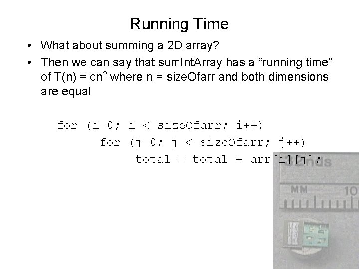
Running Time • What about summing a 2 D array? • Then we can say that sum. Int. Array has a “running time” of T(n) = cn 2 where n = size. Ofarr and both dimensions are equal for (i=0; i < size. Ofarr; i++) for (j=0; j < size. Ofarr; j++) total = total + arr[i][j];

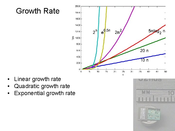
Growth Rate • Linear growth rate • Quadratic growth rate • Exponential growth rate

Best, Average, Worst • Best Case Analysis – The least amount of running time possible – The most optimistic case – Rarely of interest • Average (or typical or expected) Case Analysis – What the running time will be on the average – Requires understanding of how the universe of input data is distributed • Worst Case – The most amount of running time possible – The most pessimistic case – Provides a clear basis for comparison – Can be very important for real-time applications

Limits & Bounds • Asymptotic algorithm analysis – Interested in the resource requirements as the input size “gets big” or reaches a limit – Ignore constants • Upper Bounds – The highest growth rate that an algorithm can have. – Not the same as worst case, but the upper bound for the growth rate expressed as an equation: “this algorithm has an upper bound to its growth rate of n 2 in the worst case”

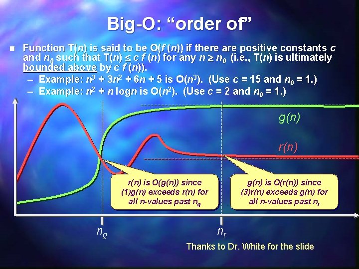
Big-O: “order of” n Function T(n) is said to be O(f (n)) if there are positive constants c and n 0 such that T(n) c f (n) for any n n 0 (i. e. , T(n) is ultimately bounded above by c f (n)). – Example: n 3 + 3 n 2 + 6 n + 5 is O(n 3). (Use c = 15 and n 0 = 1. ) – Example: n 2 + n logn is O(n 2). (Use c = 2 and n 0 = 1. ) g(n) r(n) is O(g(n)) since (1)g(n) exceeds r(n) for all n-values past ng ng g(n) is O(r(n)) since (3)r(n) exceeds g(n) for all n-values past nr nr Thanks to Dr. White for the slide

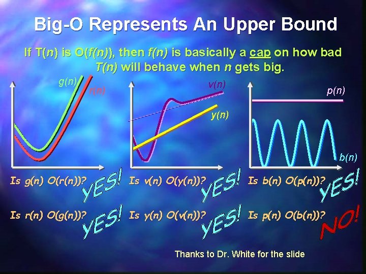
Big-O Represents An Upper Bound If T(n) is O(f(n)), then f(n) is basically a cap on how bad T(n) will behave when n gets big. g(n) v(n) r(n) p(n) y(n) b(n) Is g(n) O(r(n))? Is v(n) O(y(n))? Is b(n) O(p(n))? Is r(n) O(g(n))? Is y(n) O(v(n))? Is p(n) O(b(n))? Thanks to Dr. White for the slide

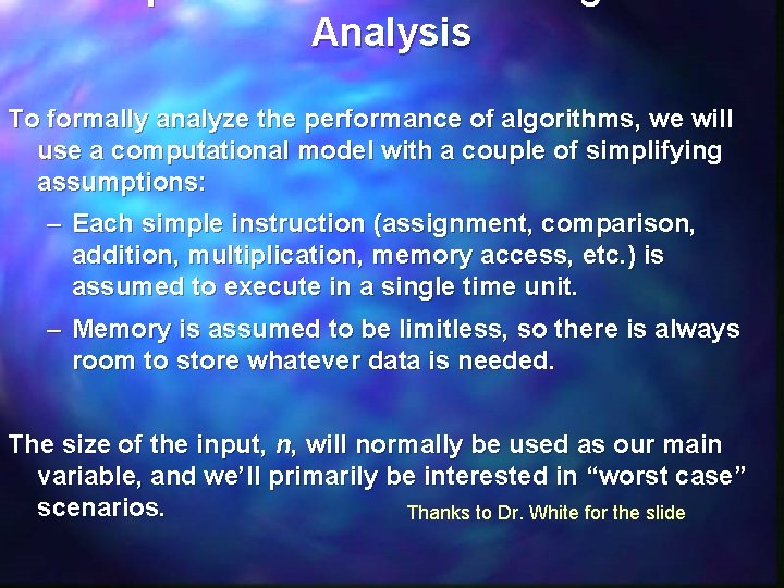
Computational Model For Algorithm Analysis To formally analyze the performance of algorithms, we will use a computational model with a couple of simplifying assumptions: – Each simple instruction (assignment, comparison, addition, multiplication, memory access, etc. ) is assumed to execute in a single time unit. – Memory is assumed to be limitless, so there is always room to store whatever data is needed. The size of the input, n, will normally be used as our main variable, and we’ll primarily be interested in “worst case” scenarios. Thanks to Dr. White for the slide

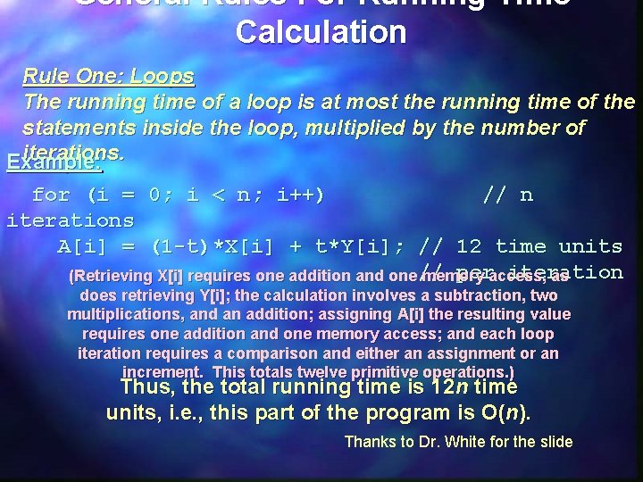
General Rules For Running Time Calculation Rule One: Loops The running time of a loop is at most the running time of the statements inside the loop, multiplied by the number of iterations. Example: for (i = 0; i < n; i++) // n iterations A[i] = (1 -t)*X[i] + t*Y[i]; // 12 time units peraccess, iteration (Retrieving X[i] requires one addition and one // memory as does retrieving Y[i]; the calculation involves a subtraction, two multiplications, and an addition; assigning A[i] the resulting value requires one addition and one memory access; and each loop iteration requires a comparison and either an assignment or an increment. This totals twelve primitive operations. ) Thus, the total running time is 12 n time units, i. e. , this part of the program is O(n). Thanks to Dr. White for the slide

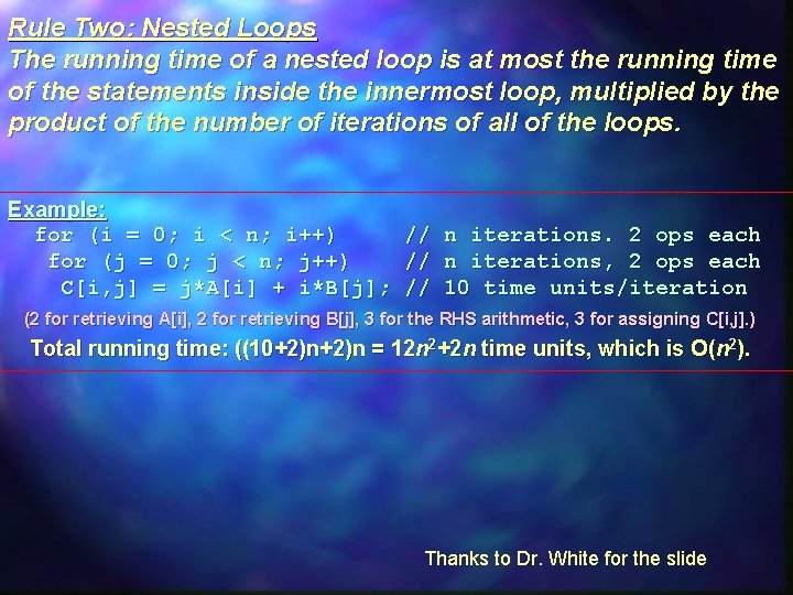
Rule Two: Nested Loops The running time of a nested loop is at most the running time of the statements inside the innermost loop, multiplied by the product of the number of iterations of all of the loops. Example: for (i = 0; i < n; i++) for (j = 0; j < n; j++) C[i, j] = j*A[i] + i*B[j]; // // // n iterations. 2 ops each n iterations, 2 ops each 10 time units/iteration (2 for retrieving A[i], 2 for retrieving B[j], 3 for the RHS arithmetic, 3 for assigning C[i, j]. ) Total running time: ((10+2)n = 12 n 2+2 n time units, which is O(n 2). Thanks to Dr. White for the slide

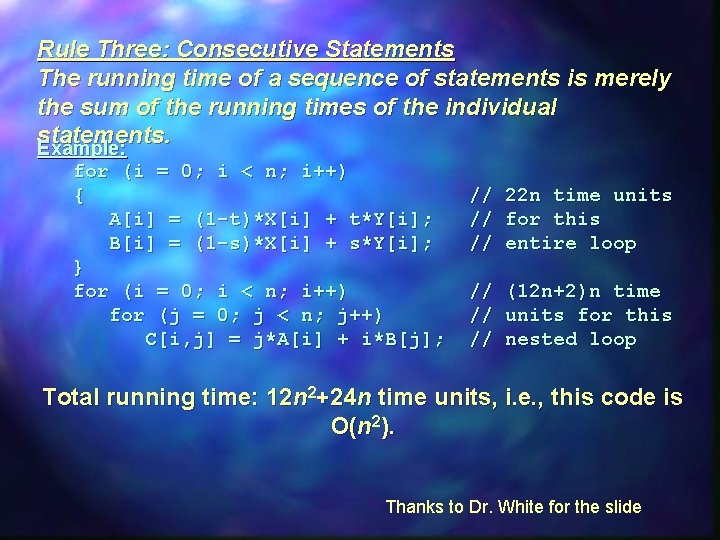
Rule Three: Consecutive Statements The running time of a sequence of statements is merely the sum of the running times of the individual statements. Example: for (i = 0; i < n; i++) { A[i] = (1 -t)*X[i] + t*Y[i]; B[i] = (1 -s)*X[i] + s*Y[i]; } for (i = 0; i < n; i++) for (j = 0; j < n; j++) C[i, j] = j*A[i] + i*B[j]; // 22 n time units // for this // entire loop // (12 n+2)n time // units for this // nested loop Total running time: 12 n 2+24 n time units, i. e. , this code is O(n 2). Thanks to Dr. White for the slide

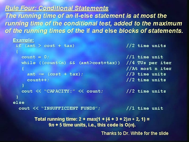
Rule Four: Conditional Statements The running time of an if-else statement is at most the running time of the conditional test, added to the maximum of the running times of the if and else blocks of statements. Example: if (amt > cost + tax) { count = 0; while ((count<n) && (amt>cost+tax)) { amt -= (cost + tax); count++; } cout << “CAPACITY: ” << count; } else cout << “INSUFFICIENT FUNDS”; //2 time units //1 time unit //4 TUs per iter //At most n iter //3 time units //2 time units //1 time unit Total running time: 2 + max(1 + (4 + 3 + 2)n + 2, 1) = 9 n + 5 time units, i. e. , this code is O(n). Thanks to Dr. White for the slide

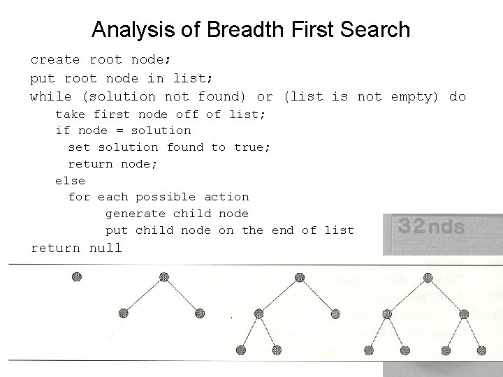
Analysis of Breadth First Search create root node; put root node in list; while (solution not found) or (list is not empty) do take first node off of list; if node = solution set solution found to true; return node; else for each possible action generate child node put child node on the end of list return null

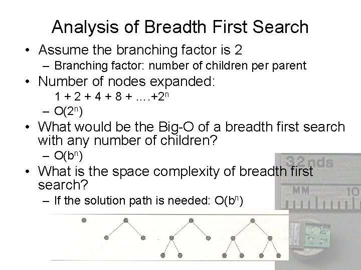
Analysis of Breadth First Search • Assume the branching factor is 2 – Branching factor: number of children per parent • Number of nodes expanded: 1 + 2 + 4 + 8 + …. +2 n – O(2 n) • What would be the Big-O of a breadth first search with any number of children? – O(bn) • What is the space complexity of breadth first search? – If the solution path is needed: O(bn)

Analysis of Depth First Search create root node; put root node in list; while (solution not found) or (list is not empty do) take first node off of list; if node = solution set solution found to true; return node; else for each possible action generate child node put child node on the start of list return null

Analysis of Depth First Search

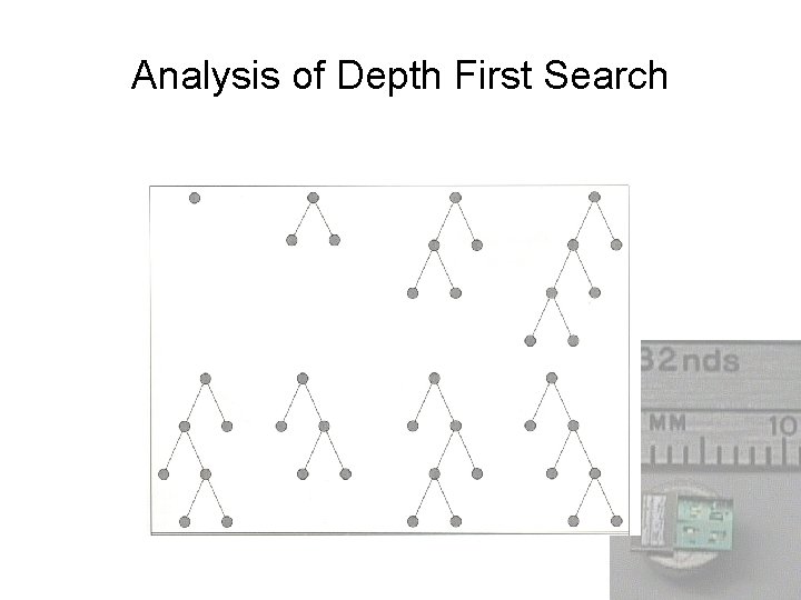
Analysis of Depth First Search • Assume the branching factor is 2 – O(2 n) • What would be the Big-O of a depth first search with any number of children? – O(bn) • What is the space complexity of depth first search? – If the solution path is needed: O(bn)

Algorithm Analysis Questions • What is the Big-O of wave front path planning? • What is the Big-O of thresholding an image to find a specific color blob?