Review Tree search Initialize the frontier using the

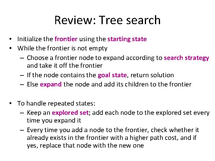
Review: Tree search • Initialize the frontier using the starting state • While the frontier is not empty – Choose a frontier node to expand according to search strategy and take it off the frontier – If the node contains the goal state, return solution – Else expand the node and add its children to the frontier • To handle repeated states: – Keep an explored set; add each node to the explored set every time you expand it – Every time you add a node to the frontier, check whether it already exists in the frontier with a higher path cost, and if yes, replace that node with the new one

Review: Uninformed search strategies • • Breadth-first search Depth-first search Iterative deepening search Uniform-cost search

Informed search strategies (Sections 3. 5 -3. 6) • Idea: give the algorithm “hints” about the desirability of different states – Use an evaluation function to rank nodes and select the most promising one for expansion • Greedy best-first search • A* search

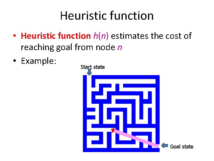
Heuristic function • Heuristic function h(n) estimates the cost of reaching goal from node n • Example: Start state Goal state

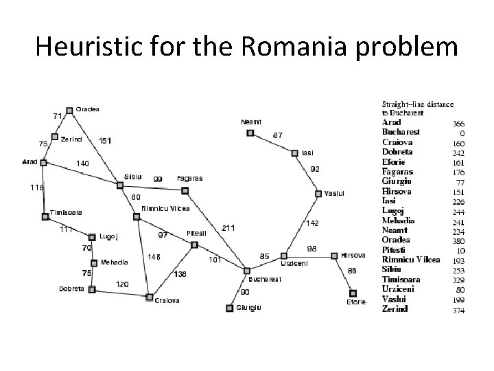
Heuristic for the Romania problem

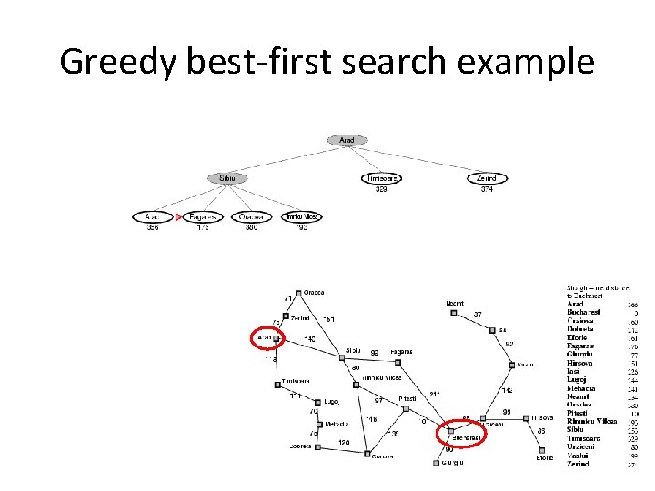
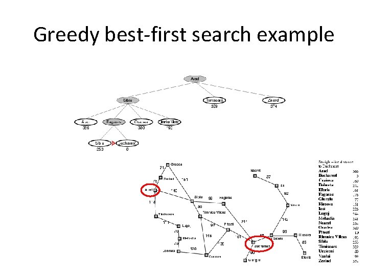
Greedy best-first search • Expand the node that has the lowest value of the heuristic function h(n)

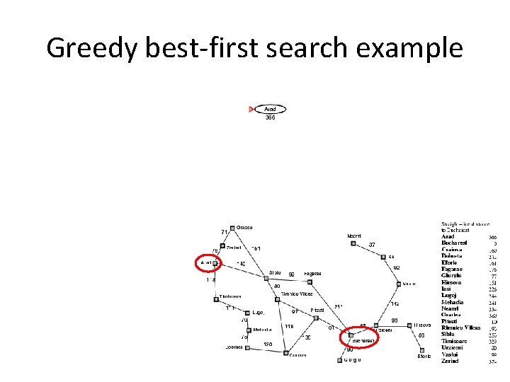
Greedy best-first search example

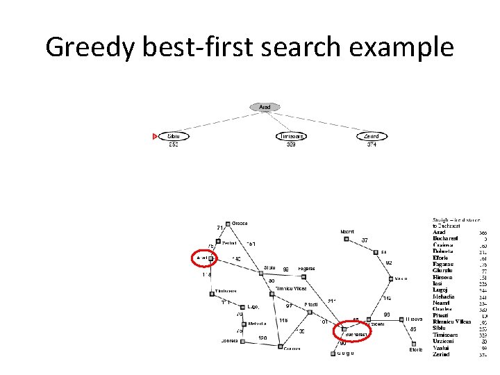
Greedy best-first search example

Greedy best-first search example

Greedy best-first search example

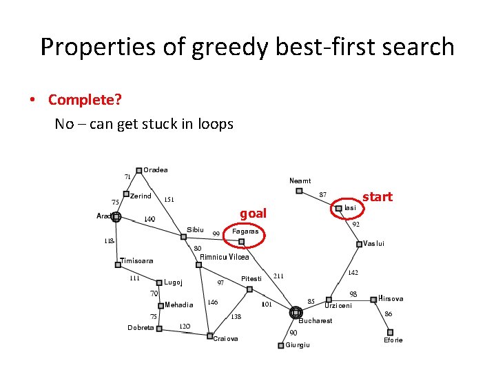
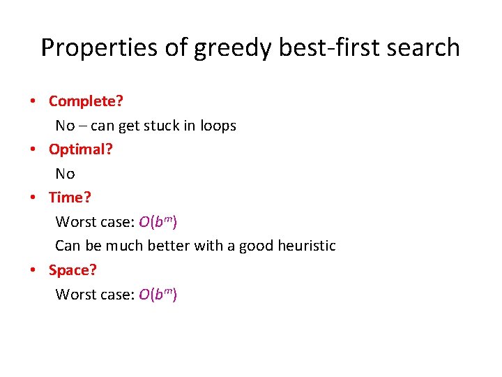
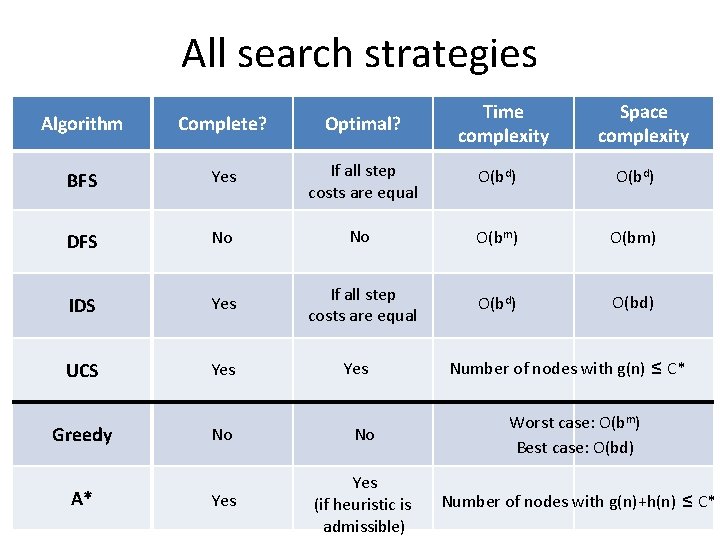
Properties of greedy best-first search • Complete? No – can get stuck in loops start goal

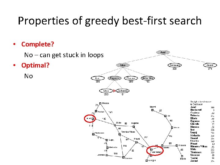
Properties of greedy best-first search • Complete? No – can get stuck in loops • Optimal? No

Properties of greedy best-first search • Complete? No – can get stuck in loops • Optimal? No • Time? Worst case: O(bm) Can be much better with a good heuristic • Space? Worst case: O(bm)

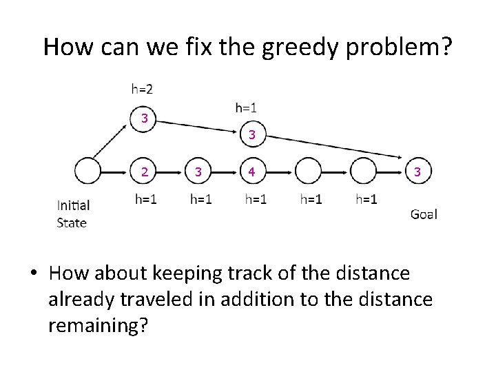
How can we fix the greedy problem? 3 3 2 3 4 3 • How about keeping track of the distance already traveled in addition to the distance remaining?

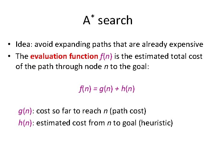
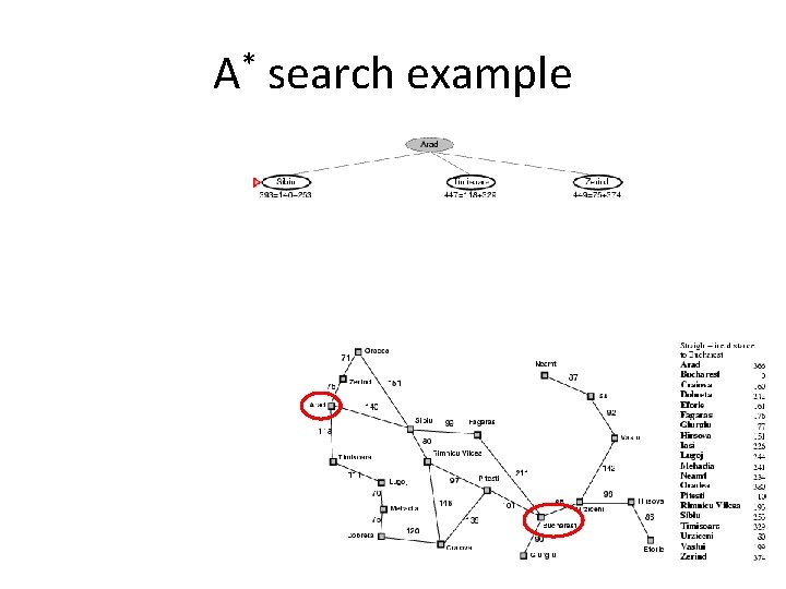
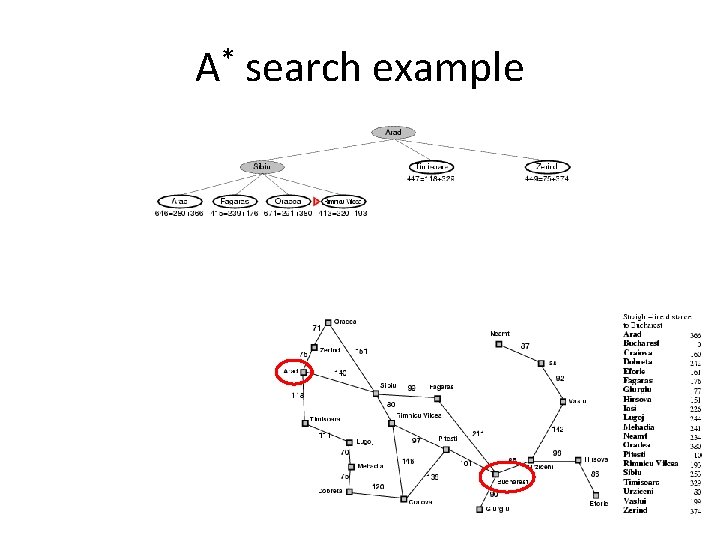
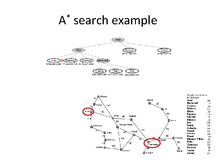
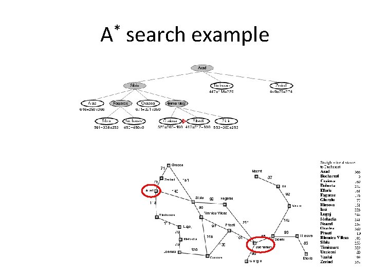
A* search • Idea: avoid expanding paths that are already expensive • The evaluation function f(n) is the estimated total cost of the path through node n to the goal: f(n) = g(n) + h(n) g(n): cost so far to reach n (path cost) h(n): estimated cost from n to goal (heuristic)

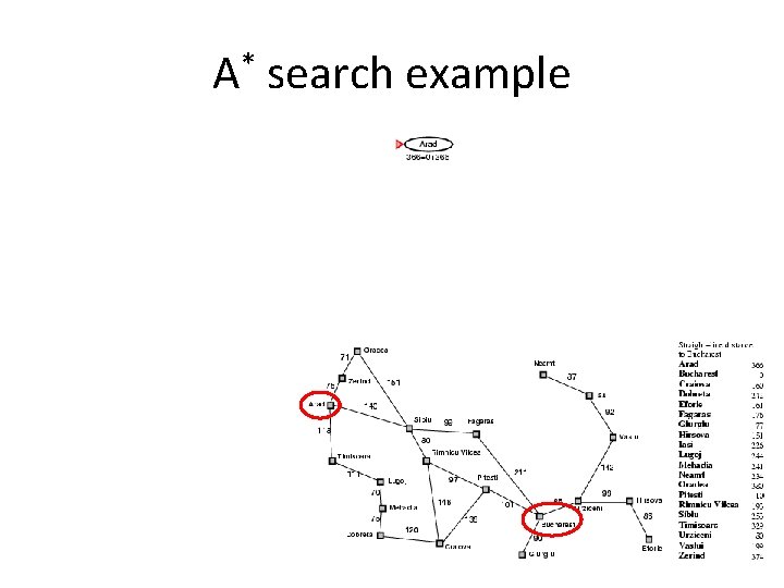
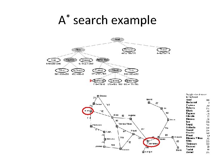
A* search example

A* search example

A* search example

A* search example

A* search example

A* search example

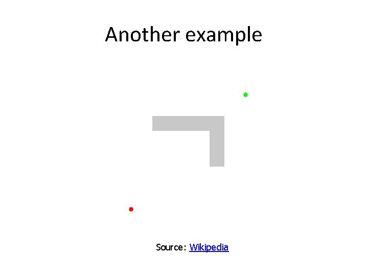
Another example Source: Wikipedia

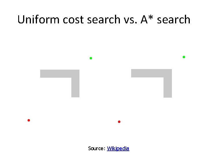
Uniform cost search vs. A* search Source: Wikipedia

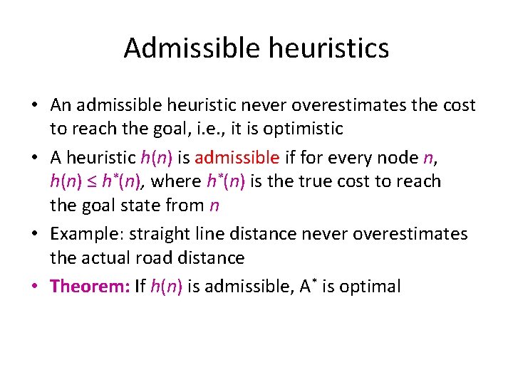
Admissible heuristics • An admissible heuristic never overestimates the cost to reach the goal, i. e. , it is optimistic • A heuristic h(n) is admissible if for every node n, h(n) ≤ h*(n), where h*(n) is the true cost to reach the goal state from n • Example: straight line distance never overestimates the actual road distance • Theorem: If h(n) is admissible, A* is optimal

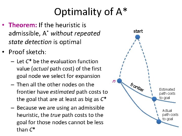
Optimality of A* • Theorem: If the heuristic is admissible, A* without repeated state detection is optimal • Proof sketch: – Let C* be the evaluation function value (actual path cost) of the first goal node we select for expansion – Then all the other nodes on the frontier have estimated path costs to the goal that are at least as big as C* – Because we are using an admissible heuristic, the true path costs to the goal for those nodes cannot be less than C* start n fro ntie r Estimated path costs to goal Actual path costs to goal

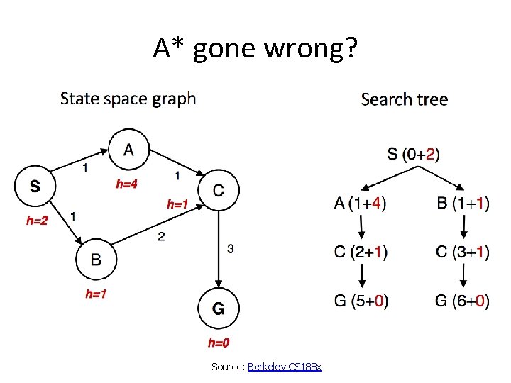
A* gone wrong? Source: Berkeley CS 188 x

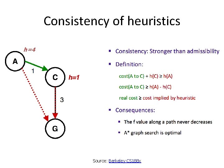
Consistency of heuristics h=4 Source: Berkeley CS 188 x

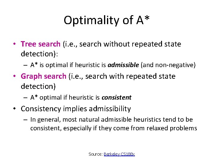
Optimality of A* • Tree search (i. e. , search without repeated state detection): – A* is optimal if heuristic is admissible (and non-negative) • Graph search (i. e. , search with repeated state detection) – A* optimal if heuristic is consistent • Consistency implies admissibility – In general, most natural admissible heuristics tend to be consistent, especially if they come from relaxed problems Source: Berkeley CS 188 x

Optimality of A* • A* is optimally efficient – no other tree-based algorithm that uses the same heuristic can expand fewer nodes and still be guaranteed to find the optimal solution – A* expands all nodes for which f(n) ≤ C*. Any algorithm that does not risks missing the optimal solution

Properties of A* • Complete? Yes – unless there are infinitely many nodes with f(n) ≤ C* • Optimal? Yes • Time? Number of nodes for which f(n) ≤ C* (exponential) • Space? Exponential

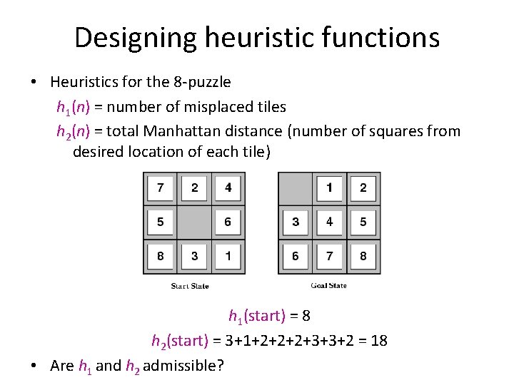
Designing heuristic functions • Heuristics for the 8 -puzzle h 1(n) = number of misplaced tiles h 2(n) = total Manhattan distance (number of squares from desired location of each tile) h 1(start) = 8 h 2(start) = 3+1+2+2+2+3+3+2 = 18 • Are h 1 and h 2 admissible?

Heuristics from relaxed problems • A problem with fewer restrictions on the actions is called a relaxed problem • The cost of an optimal solution to a relaxed problem is an admissible heuristic for the original problem • If the rules of the 8 -puzzle are relaxed so that a tile can move anywhere, then h 1(n) gives the shortest solution • If the rules are relaxed so that a tile can move to any adjacent square, then h 2(n) gives the shortest solution

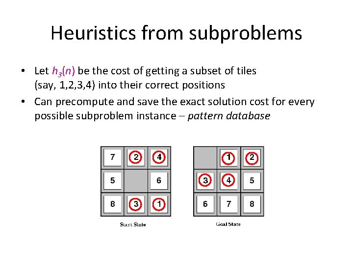
Heuristics from subproblems • Let h 3(n) be the cost of getting a subset of tiles (say, 1, 2, 3, 4) into their correct positions • Can precompute and save the exact solution cost for every possible subproblem instance – pattern database

Dominance • If h 1 and h 2 are both admissible heuristics and h 2(n) ≥ h 1(n) for all n, (both admissible) then h 2 dominates h 1 • Which one is better for search? – A* search expands every node with f(n) < C* or h(n) < C* – g(n) – Therefore, A* search with h 1 will expand more nodes

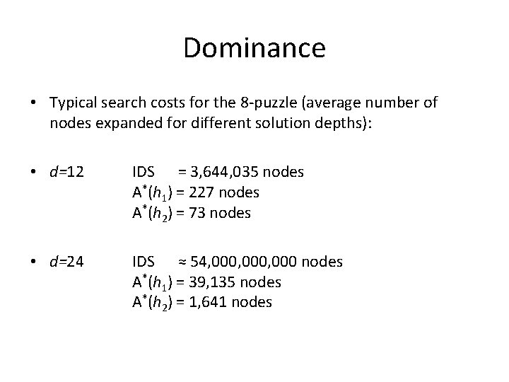
Dominance • Typical search costs for the 8 -puzzle (average number of nodes expanded for different solution depths): • d=12 IDS = 3, 644, 035 nodes A*(h 1) = 227 nodes A*(h 2) = 73 nodes • d=24 IDS ≈ 54, 000, 000 nodes A*(h 1) = 39, 135 nodes A*(h 2) = 1, 641 nodes

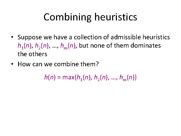
Combining heuristics • Suppose we have a collection of admissible heuristics h 1(n), h 2(n), …, hm(n), but none of them dominates the others • How can we combine them? h(n) = max{h 1(n), h 2(n), …, hm(n)}

Weighted A* search • Idea: speed up search at the expense of optimality • Take an admissible heuristic, “inflate” it by a multiple α > 1, and then perform A* search as usual • Fewer nodes tend to get expanded, but the resulting solution may be suboptimal (its cost will be at most α times the cost of the optimal solution)

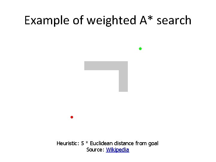
Example of weighted A* search Heuristic: 5 * Euclidean distance from goal Source: Wikipedia

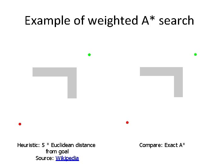
Example of weighted A* search Heuristic: 5 * Euclidean distance from goal Source: Wikipedia Compare: Exact A*

Additional pointers • Interactive path finding demo • Variants of A* for path finding on grids

All search strategies Time complexity Space complexity Algorithm Complete? Optimal? BFS Yes If all step costs are equal O(bd) DFS No No O(bm) IDS Yes If all step costs are equal O(bd) UCS Yes Greedy A* Yes Number of nodes with g(n) ≤ C* No No Worst case: O(bm) Best case: O(bd) Yes (if heuristic is admissible) Number of nodes with g(n)+h(n) ≤ C*

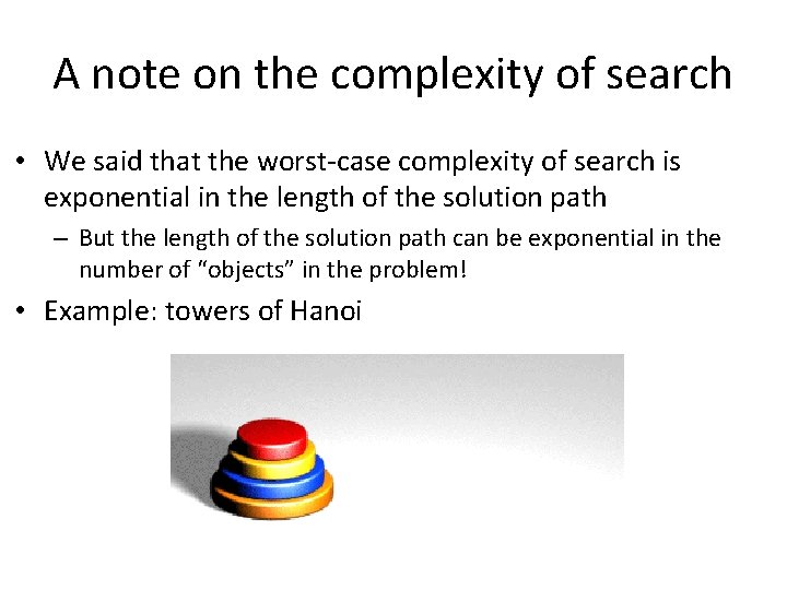
A note on the complexity of search • We said that the worst-case complexity of search is exponential in the length of the solution path – But the length of the solution path can be exponential in the number of “objects” in the problem! • Example: towers of Hanoi