Cloud Technologies and Their Applications March 26 2010

Cloud Technologies and Their Applications March 26, 2010 Indiana University Bloomington Judy Qiu xqiu@indiana. edu http: //salsahpc. indiana. edu Pervasive Technology Institute Indiana University SALSA

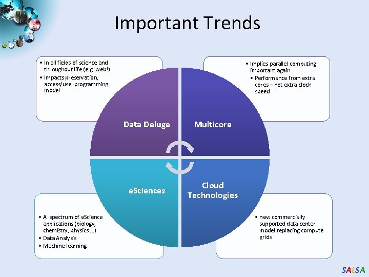
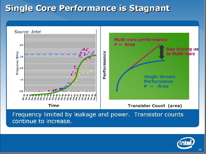
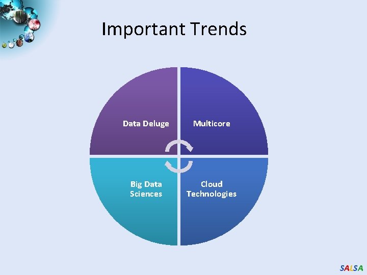
Important Trends • In all fields of science and throughout life (e. g. web!) • Impacts preservation, access/use, programming model • A spectrum of e. Science applications (biology, chemistry, physics …) • Data Analysis • Machine learning • Implies parallel computing important again • Performance from extra cores – not extra clock speed Data Deluge Multicore e. Sciences Cloud Technologies • new commercially supported data center model replacing compute grids SALSA

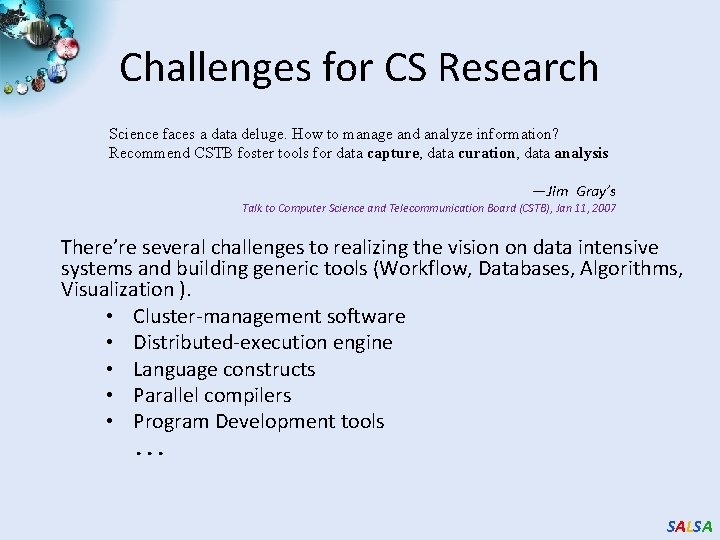
Challenges for CS Research Science faces a data deluge. How to manage and analyze information? Recommend CSTB foster tools for data capture, data curation, data analysis ―Jim Gray’s Talk to Computer Science and Telecommunication Board (CSTB), Jan 11, 2007 There’re several challenges to realizing the vision on data intensive systems and building generic tools (Workflow, Databases, Algorithms, Visualization ). • Cluster-management software • Distributed-execution engine • Language constructs • Parallel compilers • Program Development tools. . . SALSA

Important Trends Data Deluge Multicore Big Data Sciences Cloud Technologies SALSA

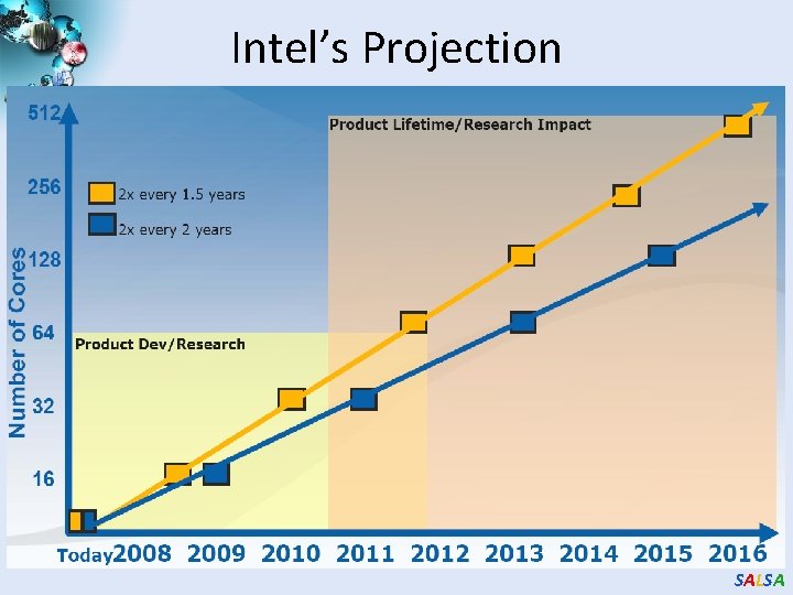
Intel’s Projection SALSA

SALSA

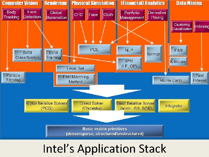
Intel’s Application Stack SALSA

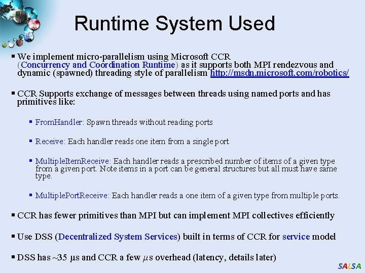
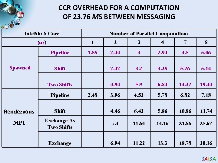
Runtime System Used § We implement micro-parallelism using Microsoft CCR (Concurrency and Coordination Runtime) as it supports both MPI rendezvous and dynamic (spawned) threading style of parallelism http: //msdn. microsoft. com/robotics/ § CCR Supports exchange of messages between threads using named ports and has primitives like: § From. Handler: Spawn threads without reading ports § Receive: Each handler reads one item from a single port § Multiple. Item. Receive: Each handler reads a prescribed number of items of a given type from a given port. Note items in a port can be general structures but all must have same type. § Multiple. Port. Receive: Each handler reads a one item of a given type from multiple ports. § CCR has fewer primitives than MPI but can implement MPI collectives efficiently § Use DSS (Decentralized System Services) built in terms of CCR for service model § DSS has ~35 µs and CCR a few µs overhead (latency, details later) SALSA

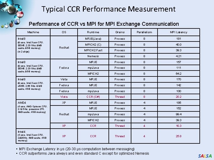
Typical CCR Performance Measurement Performance of CCR vs MPI for MPI Exchange Communication Machine OS Runtime Grains Parallelism MPI Latency MPJE(Java) Process 8 181 MPICH 2 (C) Process 8 40. 0 MPICH 2: Fast Process 8 39. 3 Nemesis Process 8 4. 21 MPJE Process 8 157 mpi. Java Process 8 111 MPICH 2 Process 8 64. 2 Vista MPJE Process 8 170 Fedora MPJE Process 8 142 Fedora mpi. Java Process 8 100 Vista CCR (C#) Thread 8 20. 2 XP MPJE Process 4 185 MPJE Process 4 152 mpi. Java Process 4 99. 4 MPICH 2 Process 4 39. 3 XP CCR Thread 4 16. 3 XP CCR Thread 4 25. 8 Intel 8 (8 core, Intel Xeon CPU, E 5345, 2. 33 Ghz, 8 MB cache, 8 GB memory) (in 2 chips) Redhat Intel 8 (8 core, Intel Xeon CPU, E 5345, 2. 33 Ghz, 8 MB cache, 8 GB memory) Intel 8 (8 core, Intel Xeon CPU, x 5355, 2. 66 Ghz, 8 MB cache, 4 GB memory) AMD 4 (4 core, AMD Opteron CPU, 2. 19 Ghz, processor 275, 4 MB cache, 4 GB memory) Fedora Redhat Intel 4 (4 core, Intel Xeon CPU, 2. 80 GHz, 4 MB cache, 4 GB memory) • MPI Exchange Latency in µs (20 -30 µs computation between messaging) • CCR outperforms Java always and even standard C except for optimized Nemesis SALSA

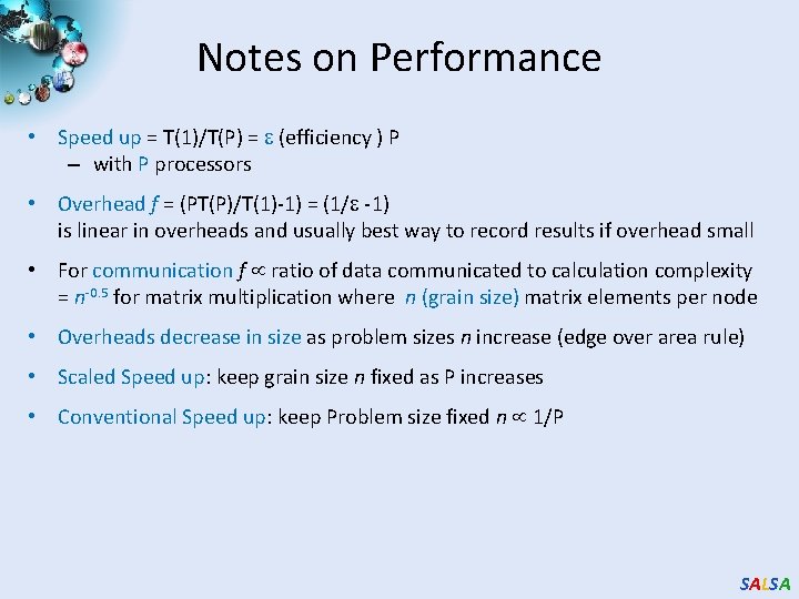
Notes on Performance • Speed up = T(1)/T(P) = (efficiency ) P – with P processors • Overhead f = (PT(P)/T(1)-1) = (1/ -1) is linear in overheads and usually best way to record results if overhead small • For communication f ratio of data communicated to calculation complexity = n-0. 5 for matrix multiplication where n (grain size) matrix elements per node • Overheads decrease in size as problem sizes n increase (edge over area rule) • Scaled Speed up: keep grain size n fixed as P increases • Conventional Speed up: keep Problem size fixed n 1/P SALSA

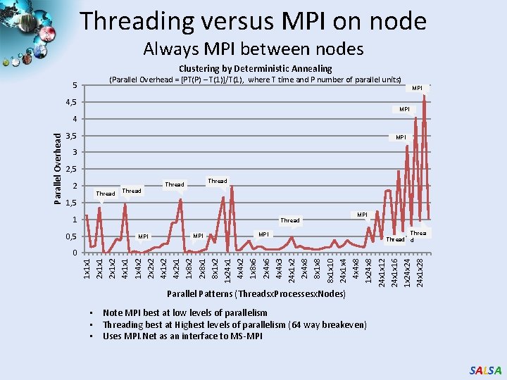
Threading versus MPI on node Always MPI between nodes Clustering by Deterministic Annealing (Parallel Overhead = [PT(P) – T(1)]/T(1), where T time and P number of parallel units) 5 MPI 4, 5 MPI 3 2, 5 2 Thread 1, 5 1 MPI Thread 0, 5 Thread d MPI MPI 24 x 1 x 28 1 x 24 24 x 1 x 16 24 x 1 x 12 1 x 24 x 8 4 x 4 x 8 24 x 1 x 4 8 x 1 x 10 8 x 1 x 8 2 x 4 x 8 24 x 1 x 2 4 x 4 x 3 2 x 4 x 6 1 x 8 x 6 4 x 4 x 2 1 x 24 x 1 8 x 1 x 2 2 x 8 x 1 1 x 8 x 2 4 x 2 x 1 4 x 1 x 2 2 x 2 x 2 1 x 4 x 2 4 x 1 x 1 2 x 1 x 2 2 x 1 x 1 0 1 x 1 x 1 Parallel Overhead 4 Parallel Patterns (Threadsx. Processesx. Nodes) • Note MPI best at low levels of parallelism • Threading best at Highest levels of parallelism (64 way breakeven) • Uses MPI. Net as an interface to MS-MPI SALSA

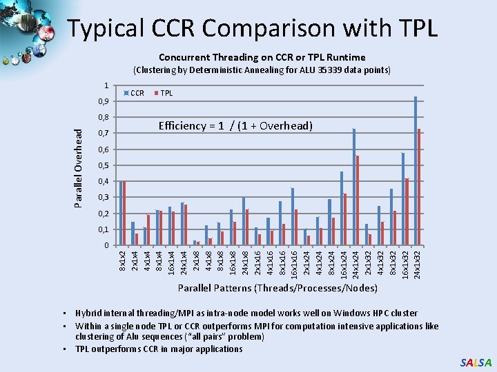
Typical CCR Comparison with TPL Concurrent Threading on CCR or TPL Runtime (Clustering by Deterministic Annealing for ALU 35339 data points) 1 0, 9 Parallel Overhead 0, 8 0, 7 CCR TPL Efficiency = 1 / (1 + Overhead) 0, 6 0, 5 0, 4 0, 3 0, 2 0, 1 8 x 1 x 2 2 x 1 x 4 4 x 1 x 4 8 x 1 x 4 16 x 1 x 4 24 x 1 x 4 2 x 1 x 8 4 x 1 x 8 8 x 1 x 8 16 x 1 x 8 24 x 1 x 8 2 x 1 x 16 4 x 1 x 16 8 x 1 x 16 16 x 1 x 16 2 x 1 x 24 4 x 1 x 24 8 x 1 x 24 16 x 1 x 24 24 x 1 x 24 2 x 1 x 32 4 x 1 x 32 8 x 1 x 32 16 x 1 x 32 24 x 1 x 32 0 Parallel Patterns (Threads/Processes/Nodes) • Hybrid internal threading/MPI as intra-node model works well on Windows HPC cluster • Within a single node TPL or CCR outperforms MPI for computation intensive applications like clustering of Alu sequences (“all pairs” problem) • TPL outperforms CCR in major applications SALSA

CCR OVERHEAD FOR A COMPUTATION OF 23. 76 ΜS BETWEEN MESSAGING Intel 8 b: 8 Core (μs) 1 2 3 4 7 8 1. 58 2. 44 3 2. 94 4. 5 5. 06 Shift 2. 42 3. 38 5. 26 5. 14 Two Shifts 4. 94 5. 9 6. 84 14. 32 19. 44 3. 96 4. 52 5. 78 6. 82 7. 18 Pipeline Spawned Number of Parallel Computations Pipeline 2. 48 Rendezvous Shift 4. 46 6. 42 5. 86 10. 86 11. 74 MPI Exchange As Two Shifts 7. 4 11. 64 14. 16 31. 86 35. 62 Exchange 6. 94 11. 22 13. 3 18. 78 20. 16 SALSA

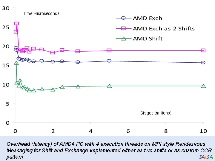
Time Microseconds Stages (millions) Overhead (latency) of AMD 4 PC with 4 execution threads on MPI style Rendezvous Messaging for Shift and Exchange implemented either as two shifts or as custom CCR SALSA pattern

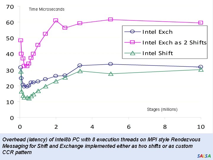
Time Microseconds Stages (millions) Overhead (latency) of Intel 8 b PC with 8 execution threads on MPI style Rendezvous Messaging for Shift and Exchange implemented either as two shifts or as custom CCR pattern SALSA

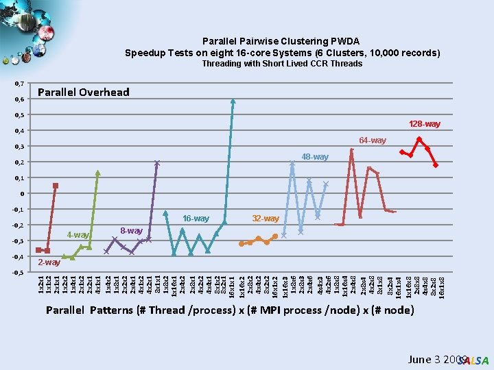
Parallel Pairwise Clustering PWDA Speedup Tests on eight 16 -core Systems (6 Clusters, 10, 000 records) Threading with Short Lived CCR Threads 0, 7 0, 6 Parallel Overhead 0, 5 128 -way 0, 4 64 -way 0, 3 48 -way 0, 2 0, 1 0 -0, 1 16 -way -0, 2 4 -way -0, 3 -0, 5 8 -way 2 -way 1 x 2 x 1 1 x 1 x 2 2 x 1 x 1 1 x 2 x 2 1 x 4 x 1 2 x 1 x 2 2 x 2 x 1 4 x 1 x 1 1 x 4 x 2 1 x 8 x 1 2 x 2 x 2 2 x 4 x 1 x 2 4 x 2 x 1 8 x 1 x 1 1 x 8 x 2 1 x 16 x 1 2 x 4 x 2 2 x 8 x 1 4 x 2 x 2 4 x 4 x 1 8 x 1 x 2 8 x 2 x 1 16 x 1 x 16 x 2 2 x 8 x 2 4 x 4 x 2 8 x 2 x 2 16 x 1 x 2 1 x 16 x 3 1 x 8 x 6 2 x 8 x 3 2 x 4 x 6 4 x 4 x 3 4 x 2 x 6 1 x 8 x 8 1 x 16 x 4 2 x 4 x 8 2 x 8 x 4 4 x 2 x 8 8 x 1 x 8 8 x 2 x 4 16 x 1 x 4 1 x 16 x 8 2 x 8 x 8 4 x 4 x 8 8 x 2 x 8 16 x 1 x 8 -0, 4 32 -way Parallel Patterns (# Thread /process) x (# MPI process /node) x (# node) June 3 2009 SALSA

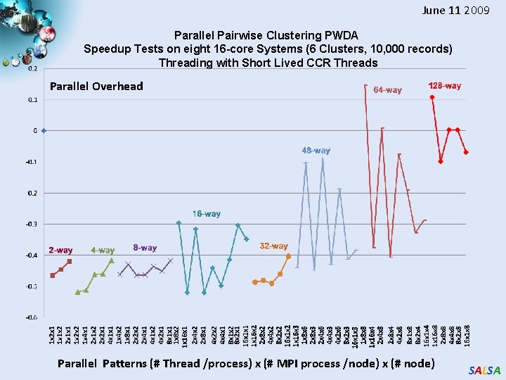
June 11 2009 Parallel Pairwise Clustering PWDA Speedup Tests on eight 16 -core Systems (6 Clusters, 10, 000 records) Threading with Short Lived CCR Threads Parallel Overhead Parallel Patterns (# Thread /process) x (# MPI process /node) x (# node) SALSA

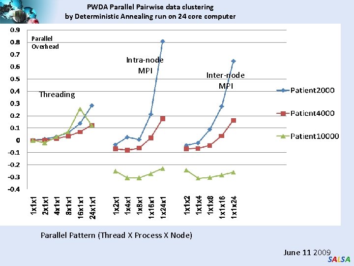
PWDA Parallel Pairwise data clustering by Deterministic Annealing run on 24 core computer Parallel Overhead Intra-node MPI Threading Inter-node MPI Parallel Pattern (Thread X Process X Node) June 11 2009 SALSA

Important Trends Data Deluge Multicore Big Data Sciences Cloud Technologies SALSA

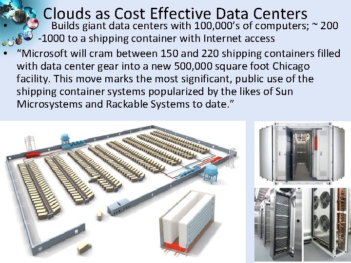
Clouds as Cost Effective Data Centers Builds giant data centers with 100, 000’s of computers; ~ 200 -1000 to a shipping container with Internet access • “Microsoft will cram between 150 and 220 shipping containers filled with data center gear into a new 500, 000 square foot Chicago facility. This move marks the most significant, public use of the shipping container systems popularized by the likes of Sun Microsystems and Rackable Systems to date. ” • 20 SALSA

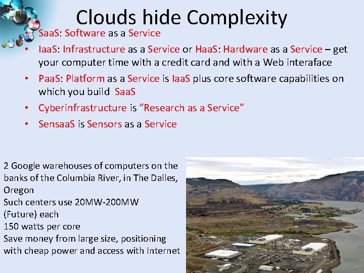
Clouds hide Complexity • Saa. S: Software as a Service • Iaa. S: Infrastructure as a Service or Haa. S: Hardware as a Service – get your computer time with a credit card and with a Web interaface • Paa. S: Platform as a Service is Iaa. S plus core software capabilities on which you build Saa. S • Cyberinfrastructure is “Research as a Service” • Sensaa. S is Sensors as a Service 2 Google warehouses of computers on the banks of the Columbia River, in The Dalles, Oregon Such centers use 20 MW-200 MW (Future) each 150 watts per core Save money from large size, positioning with cheap power and access with Internet 21 SALSA

SALSA

Philosophy of Clouds and Grids • Clouds are (by definition) commercially supported approach to large scale computing – So we should expect Clouds to replace Compute Grids – Current Grid technology involves “non-commercial” software solutions which are hard to evolve/sustain – Maybe Clouds ~4% IT expenditure 2008 growing to 14% in 2012 (IDC Estimate) • Public Clouds are broadly accessible resources like Amazon and Microsoft Azure – powerful but not easy to optimize and perhaps data trust/privacy issues • Private Clouds run similar software and mechanisms but on “your own computers” • Services still are correct architecture with either REST (Web 2. 0) or Web Services SALSA

Cloud Computing: Infrastructure and Runtimes • Cloud infrastructure: outsourcing of servers, computing, data, file space, utility computing, etc. – Handled through Web services that control virtual machine lifecycles. • Cloud runtimes: tools (for using clouds) to do data-parallel computations. – Apache Hadoop (Pig. Latin, SCOPE), Google Map. Reduce, Microsoft Dryad, and others – Designed for information retrieval but are excellent for a wide range of science data analysis applications – Can also do much traditional parallel computing for data-mining if extended to support iterative operations – Not usually on Virtual Machines SALSA

Map Reduce The Story of Sam … SALSA

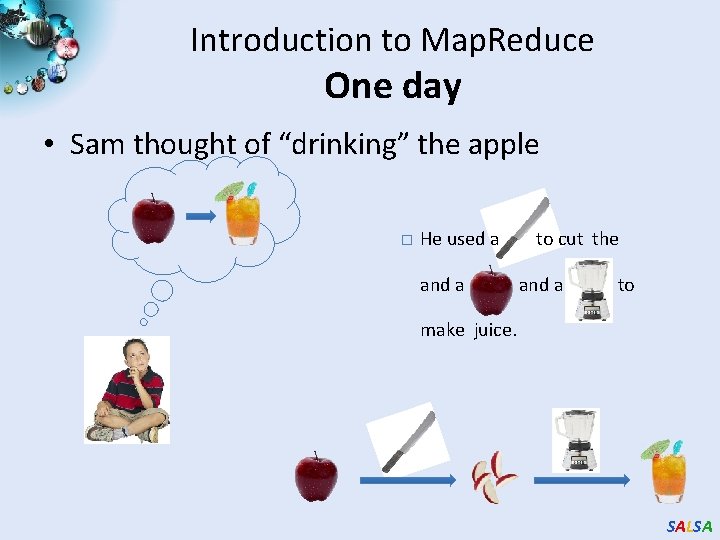
Introduction to Map. Reduce One day • Sam thought of “drinking” the apple � He used a and a to cut the and a to make juice. SALSA

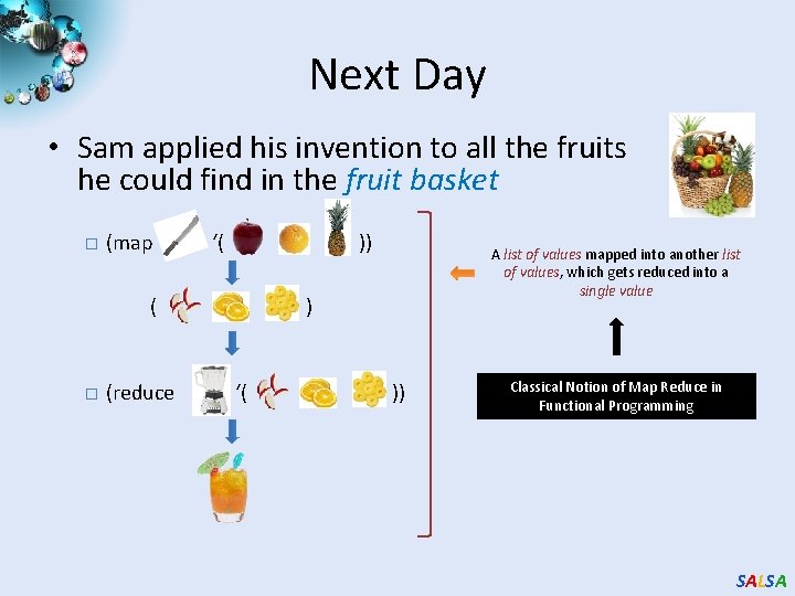
Next Day • Sam applied his invention to all the fruits he could find in the fruit basket � (map ‘( )) ( � (reduce A list of values mapped into another list of values, which gets reduced into a single value ) ‘( )) Classical Notion of Map Reduce in Functional Programming SALSA

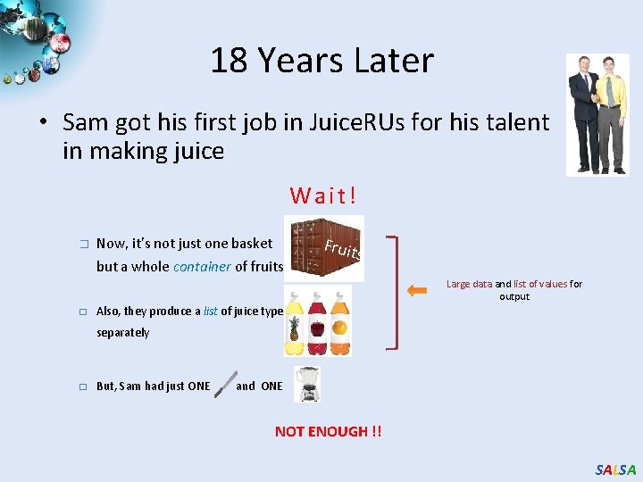
18 Years Later • Sam got his first job in Juice. RUs for his talent in making juice Wait! � Now, it’s not just one basket but a whole container of fruits Fruit s Large data and list of values for output � Also, they produce a list of juice types separately � But, Sam had just ONE and ONE NOT ENOUGH !! SALSA

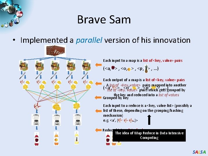
Brave Sam • Implemented a parallel version of his innovation Fruit s Each input to a map is a list of <key, value> pairs (<a, > , <o, > , <p, > , …) Each output of a map is a list of <key, value> pairs A list of <key, value> pairs mapped into another (<a’, , <o’, , <p’, , …)grouped by list of > <key, value>>pairs which>gets the key and reduced into a list of values Grouped by key Each input to a reduce is a <key, value-list> (possibly a list of these, depending on the grouping/hashing mechanism) e. g. <a’, ( …)> Reduced into a list of values The idea of Map Reduce in Data Intensive Computing SALSA

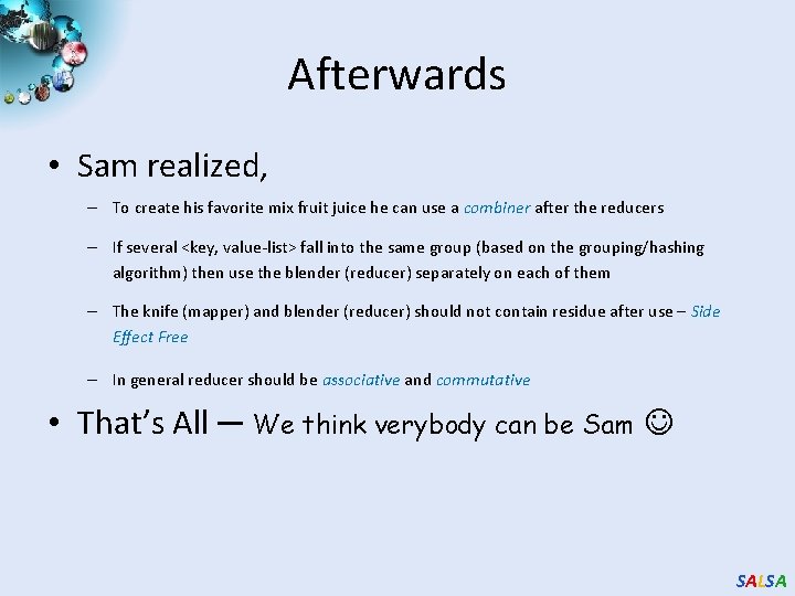
Afterwards • Sam realized, – To create his favorite mix fruit juice he can use a combiner after the reducers – If several <key, value-list> fall into the same group (based on the grouping/hashing algorithm) then use the blender (reducer) separately on each of them – The knife (mapper) and blender (reducer) should not contain residue after use – Side Effect Free – In general reducer should be associative and commutative • That’s All ─ We think verybody can be Sam SALSA

Important Trends Data Deluge Multicore Big Data Sciences Cloud Technologies SALSA

Parallel Data Analysis Algorithms on Multicore Developing a suite of parallel data-analysis capabilities § Clustering with deterministic annealing (DA) § Dimension Reduction for visualization and analysis § Matrix algebra as needed § Matrix Multiplication § Equation Solving § Eigenvector/value Calculation SALSA

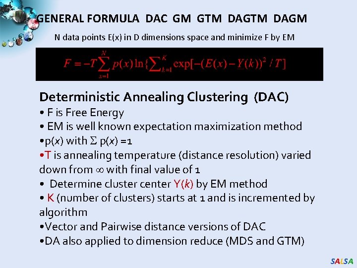
GENERAL FORMULA DAC GM GTM DAGM N data points E(x) in D dimensions space and minimize F by EM Deterministic Annealing Clustering (DAC) • F is Free Energy • EM is well known expectation maximization method • p(x) with p(x) =1 • T is annealing temperature (distance resolution) varied down from with final value of 1 • Determine cluster center Y(k) by EM method • K (number of clusters) starts at 1 and is incremented by algorithm • Vector and Pairwise distance versions of DAC • DA also applied to dimension reduce (MDS and GTM) SALSA

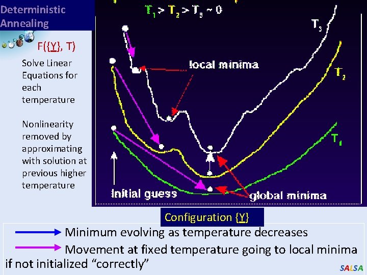
Deterministic Annealing F({Y}, T) Solve Linear Equations for each temperature Nonlinearity removed by approximating with solution at previous higher temperature Configuration {Y} Minimum evolving as temperature decreases Movement at fixed temperature going to local minima if not initialized “correctly” SALSA

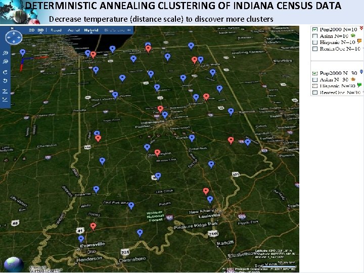
DETERMINISTIC ANNEALING CLUSTERING OF INDIANA CENSUS DATA Decrease temperature (distance scale) to discover more clusters SALSA

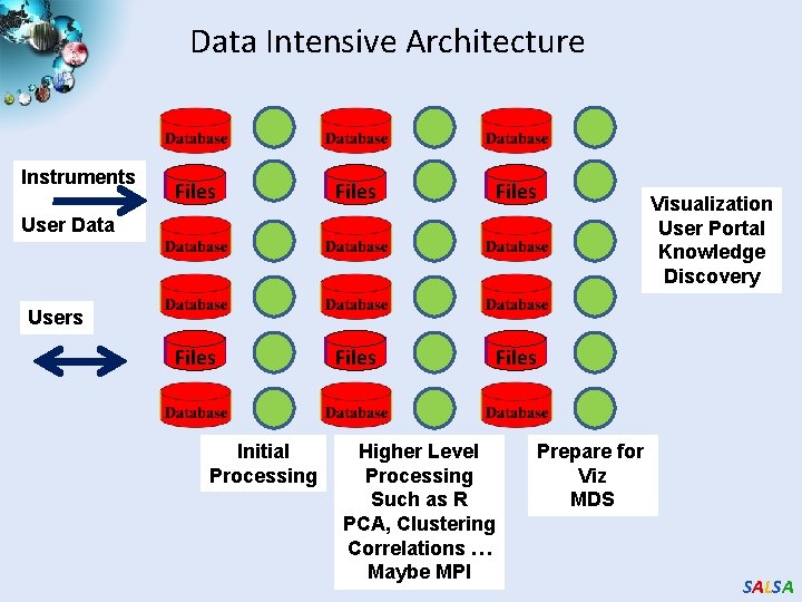
Data Intensive Architecture Instruments Files Files User Data Visualization User Portal Knowledge Discovery Users Initial Processing Higher Level Processing Such as R PCA, Clustering Correlations … Maybe MPI Prepare for Viz MDS SALSA

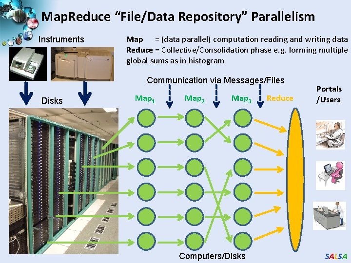
Map. Reduce “File/Data Repository” Parallelism Instruments Map = (data parallel) computation reading and writing data Reduce = Collective/Consolidation phase e. g. forming multiple global sums as in histogram Communication via Messages/Files Disks Map 1 Map 2 Map 3 Computers/Disks Reduce Portals /Users SALSA

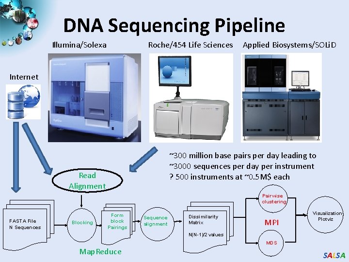
DNA Sequencing Pipeline Illumina/Solexa Roche/454 Life Sciences Applied Biosystems/SOLi. D Internet ~300 million base pairs per day leading to ~3000 sequences per day per instrument ? 500 instruments at ~0. 5 M$ each Read Alignment Pairwise clustering FASTA File N Sequences Blocking Form block Pairings Sequence alignment Dissimilarity Matrix MPI Visualization Plotviz N(N-1)/2 values MDS Map. Reduce SALSA

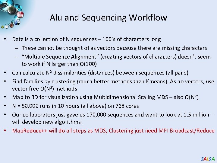
Alu and Sequencing Workflow • Data is a collection of N sequences – 100’s of characters long – These cannot be thought of as vectors because there are missing characters – “Multiple Sequence Alignment” (creating vectors of characters) doesn’t seem to work if N larger than O(100) • Can calculate N 2 dissimilarities (distances) between sequences (all pairs) • Find families by clustering (much better methods than Kmeans). As no vectors, use vector free O(N 2) methods • Map to 3 D for visualization using Multidimensional Scaling MDS – also O(N 2) • N = 50, 000 runs in 10 hours (all above) on 768 cores • Our collaborators just gave us 170, 000 sequences and want to look at 1. 5 million – will develop new algorithms! • Map. Reduce++ will do all steps as MDS, Clustering just need MPI Broadcast/Reduce SALSA

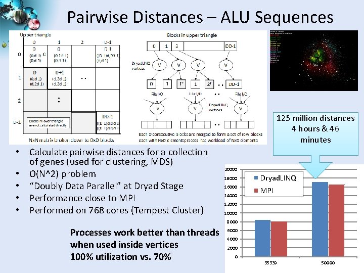
Pairwise Distances – ALU Sequences 125 million distances 4 hours & 46 minutes • Calculate pairwise distances for a collection of genes (used for clustering, MDS) • O(N^2) problem • “Doubly Data Parallel” at Dryad Stage • Performance close to MPI • Performed on 768 cores (Tempest Cluster) 20000 18000 Dryad. LINQ 16000 MPI 14000 12000 10000 8000 Processes work better than threads when used inside vertices 100% utilization vs. 70% 6000 4000 2000 0 35339 50000 SALSA

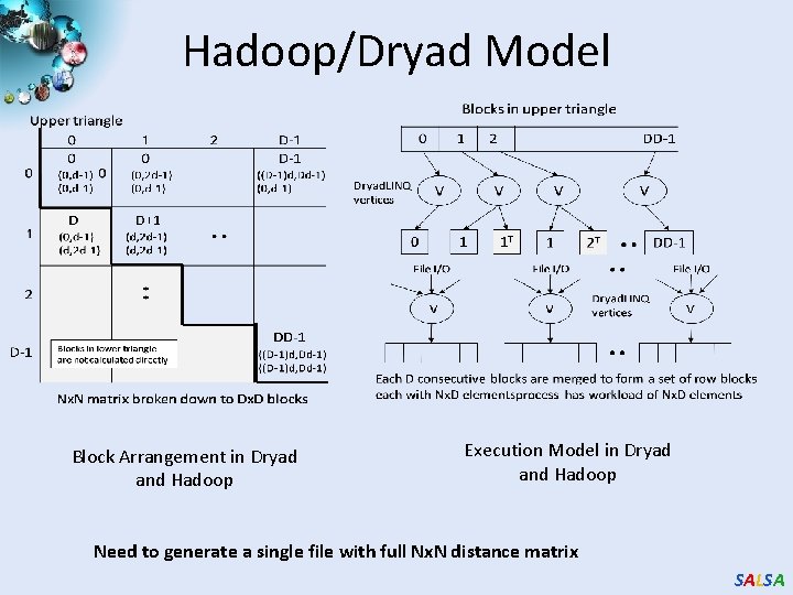
Hadoop/Dryad Model Block Arrangement in Dryad and Hadoop Execution Model in Dryad and Hadoop Need to generate a single file with full Nx. N distance matrix SALSA

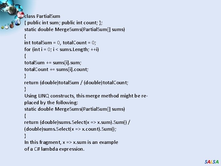
class Partial. Sum { public int sum; public int count; }; static double Merge. Sums(Partial. Sum[] sums) { int total. Sum = 0, total. Count = 0; for (int i = 0; i < sums. Length; ++i) { total. Sum += sums[i]. sum; total. Count += sums[i]. count; } return (double)total. Sum / (double)total. Count; } Using LINQ constructs, this merge method might be replaced by the following: static double Merge. Sums(Partial. Sum[] sums) { return (double)sums. Select(x => x. sum). Sum() / (double)sums. Select(x => x. count). Sum(); } In this fragment, x => x. sum is an example of a C# lambda expression. SALSA

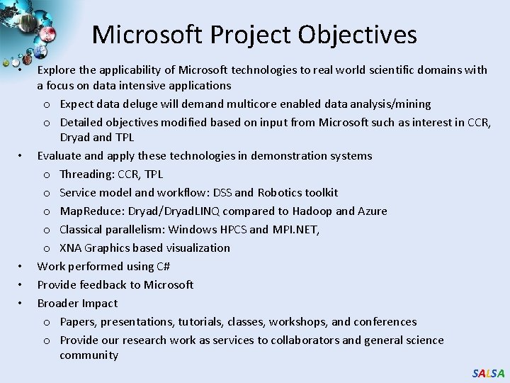
Microsoft Project Objectives • • • Explore the applicability of Microsoft technologies to real world scientific domains with a focus on data intensive applications o Expect data deluge will demand multicore enabled data analysis/mining o Detailed objectives modified based on input from Microsoft such as interest in CCR, Dryad and TPL Evaluate and apply these technologies in demonstration systems o Threading: CCR, TPL o Service model and workflow: DSS and Robotics toolkit o Map. Reduce: Dryad/Dryad. LINQ compared to Hadoop and Azure o Classical parallelism: Windows HPCS and MPI. NET, o XNA Graphics based visualization Work performed using C# Provide feedback to Microsoft Broader Impact o Papers, presentations, tutorials, classes, workshops, and conferences o Provide our research work as services to collaborators and general science community SALSA

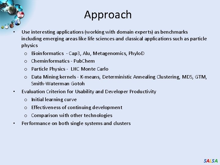
Approach • • • Use interesting applications (working with domain experts) as benchmarks including emerging areas like life sciences and classical applications such as particle physics o Bioinformatics - Cap 3, Alu, Metagenomics, Phylo. D o Cheminformatics - Pub. Chem o Particle Physics - LHC Monte Carlo o Data Mining kernels - K-means, Deterministic Annealing Clustering, MDS, GTM, Smith-Waterman Gotoh Evaluation Criterion for Usability and Developer Productivity o Initial learning curve o Effectiveness of continuing development o Comparison with other technologies Performance on both single systems and clusters SALSA

Overview of Multicore SALSA Project at IU • The term SALSA or Service Aggregated Linked Sequential Activities, describes our approach to multicore computing where we used services as modules to capture key functionalities implemented with multicore threading. o This will be expanded as a proposed approach to parallel computing where one produces libraries of parallelized components and combines them with a generalized service integration (workflow) model • We have adopted a multi-paradigm runtime (MPR) approach to support key parallel models with focus on Map. Reduce, MPI collective messaging, asynchronous threading, coarse grain functional parallelism or workflow. • We have developed innovative data mining algorithms emphasizing robustness essential for data intensive applications. Parallel algorithms have been developed for shared memory threading, tightly coupled clusters and distributed environments. These have been demonstrated in kernel and real applications. SALSA

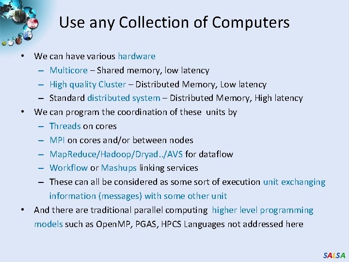
Use any Collection of Computers • We can have various hardware – Multicore – Shared memory, low latency – High quality Cluster – Distributed Memory, Low latency – Standard distributed system – Distributed Memory, High latency • We can program the coordination of these units by – Threads on cores – MPI on cores and/or between nodes – Map. Reduce/Hadoop/Dryad. . /AVS for dataflow – Workflow or Mashups linking services – These can all be considered as some sort of execution unit exchanging information (messages) with some other unit • And there are traditional parallel computing higher level programming models such as Open. MP, PGAS, HPCS Languages not addressed here SALSA

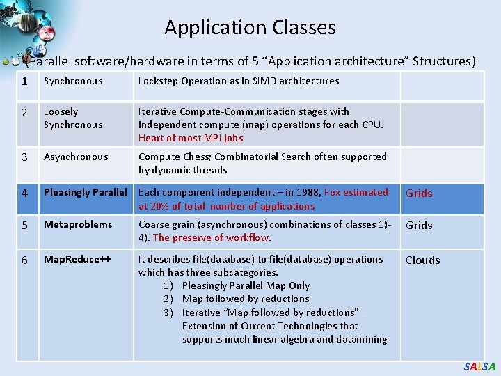
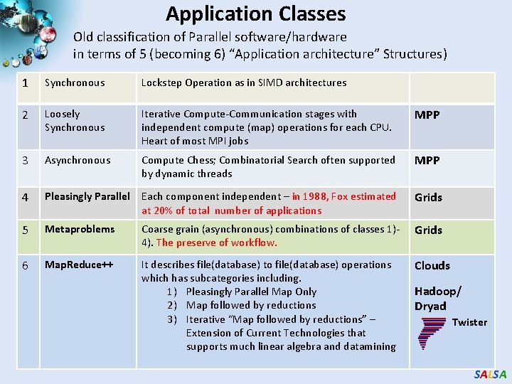
Application Classes (Parallel software/hardware in terms of 5 “Application architecture” Structures) 1 Synchronous Lockstep Operation as in SIMD architectures 2 Loosely Synchronous Iterative Compute-Communication stages with independent compute (map) operations for each CPU. Heart of most MPI jobs 3 Asynchronous Compute Chess; Combinatorial Search often supported by dynamic threads 4 Pleasingly Parallel Each component independent – in 1988, Fox estimated at 20% of total number of applications Grids 5 Metaproblems Coarse grain (asynchronous) combinations of classes 1)4). The preserve of workflow. Grids 6 Map. Reduce++ It describes file(database) to file(database) operations which has three subcategories. 1) Pleasingly Parallel Map Only 2) Map followed by reductions 3) Iterative “Map followed by reductions” – Extension of Current Technologies that supports much linear algebra and datamining Clouds SALSA

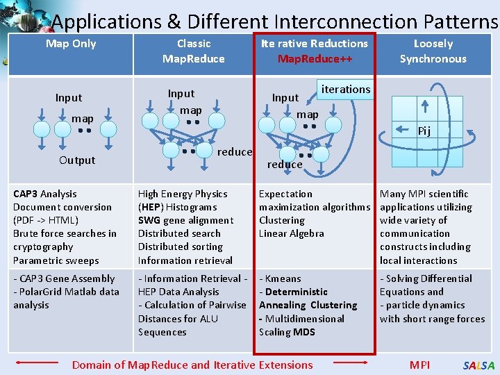
Applications & Different Interconnection Patterns Map Only Input map Output Classic Map. Reduce Input map Ite rative Reductions Map. Reduce++ Input map Loosely Synchronous iterations Pij reduce CAP 3 Analysis Document conversion (PDF -> HTML) Brute force searches in cryptography Parametric sweeps High Energy Physics (HEP) Histograms SWG gene alignment Distributed search Distributed sorting Information retrieval Expectation maximization algorithms Clustering Linear Algebra Many MPI scientific applications utilizing wide variety of communication constructs including local interactions - CAP 3 Gene Assembly - Polar. Grid Matlab data analysis - Information Retrieval HEP Data Analysis - Calculation of Pairwise Distances for ALU Sequences - Kmeans - Deterministic Annealing Clustering - Multidimensional Scaling MDS - Solving Differential Equations and - particle dynamics with short range forces Domain of Map. Reduce and Iterative Extensions MPI SALSA

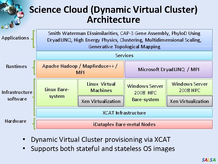
Science Cloud (Dynamic Virtual Cluster) Architecture Applications Smith Waterman Dissimilarities, CAP-3 Gene Assembly, Phylo. D Using Dryad. LINQ, High Energy Physics, Clustering, Multidimensional Scaling, Generative Topological Mapping Services Runtimes Infrastructure software Apache Hadoop / Map. Reduce++ / MPI Linux Baresystem Linux Virtual Machines Xen Virtualization Microsoft Dryad. LINQ / MPI Windows Server 2008 HPC Bare-system Windows Server 2008 HPC Xen Virtualization XCAT Infrastructure Hardware i. Dataplex Bare-metal Nodes • Dynamic Virtual Cluster provisioning via XCAT • Supports both stateful and stateless OS images SALSA

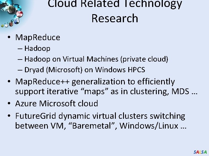
Cloud Related Technology Research • Map. Reduce – Hadoop on Virtual Machines (private cloud) – Dryad (Microsoft) on Windows HPCS • Map. Reduce++ generalization to efficiently support iterative “maps” as in clustering, MDS … • Azure Microsoft cloud • Future. Grid dynamic virtual clusters switching between VM, “Baremetal”, Windows/Linux … SALSA

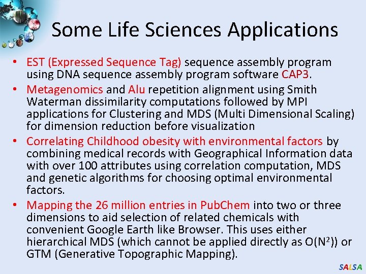
Some Life Sciences Applications • EST (Expressed Sequence Tag) sequence assembly program using DNA sequence assembly program software CAP 3. • Metagenomics and Alu repetition alignment using Smith Waterman dissimilarity computations followed by MPI applications for Clustering and MDS (Multi Dimensional Scaling) for dimension reduction before visualization • Correlating Childhood obesity with environmental factors by combining medical records with Geographical Information data with over 100 attributes using correlation computation, MDS and genetic algorithms for choosing optimal environmental factors. • Mapping the 26 million entries in Pub. Chem into two or three dimensions to aid selection of related chemicals with convenient Google Earth like Browser. This uses either hierarchical MDS (which cannot be applied directly as O(N 2)) or GTM (Generative Topographic Mapping). SALSA

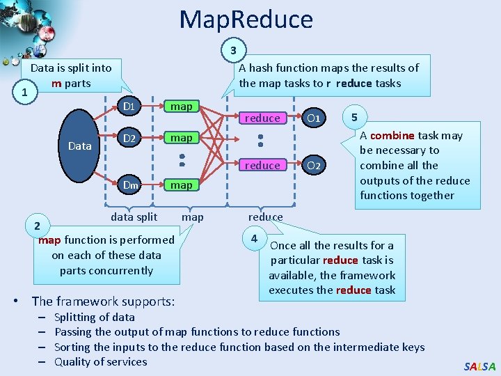
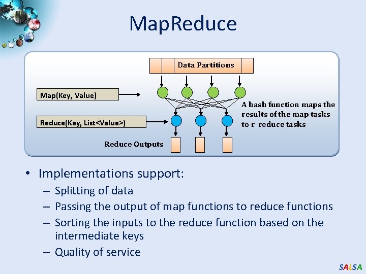
Map. Reduce 3 1 Data is split into m parts Data A hash function maps the results of the map tasks to r reduce tasks D 1 map D 2 map reduce Dm map data split map 2 map function is performed on each of these data parts concurrently • The framework supports: – – O 1 O 2 5 A combine task may be necessary to combine all the outputs of the reduce functions together reduce 4 Once all the results for a particular reduce task is available, the framework executes the reduce task Splitting of data Passing the output of map functions to reduce functions Sorting the inputs to the reduce function based on the intermediate keys Quality of services SALSA

Map. Reduce Data Partitions Map(Key, Value) Reduce(Key, List<Value>) A hash function maps the results of the map tasks to r reduce tasks Reduce Outputs • Implementations support: – Splitting of data – Passing the output of map functions to reduce functions – Sorting the inputs to the reduce function based on the intermediate keys – Quality of service SALSA

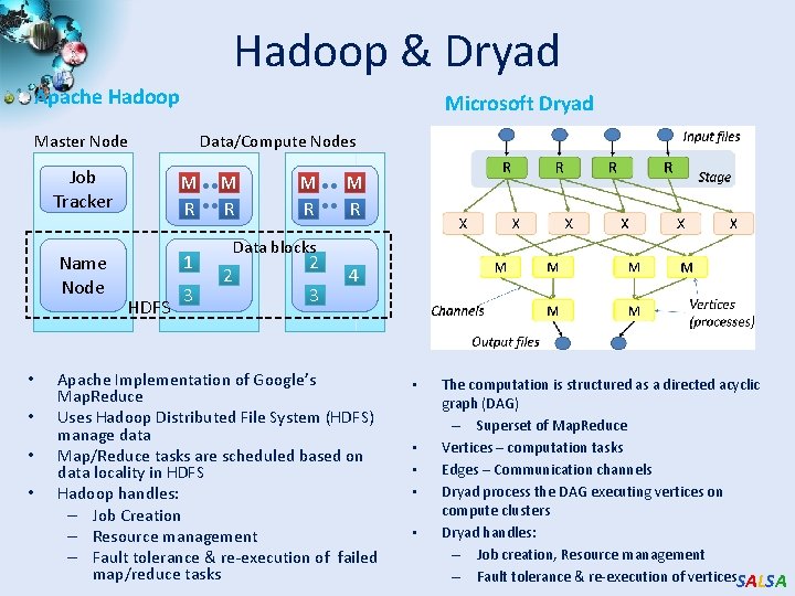
Hadoop & Dryad Apache Hadoop Microsoft Dryad Master Node • • Data/Compute Nodes Job Tracker M R Name Node 1 HDFS 3 M R M R Data blocks 2 2 3 4 Apache Implementation of Google’s Map. Reduce Uses Hadoop Distributed File System (HDFS) manage data Map/Reduce tasks are scheduled based on data locality in HDFS Hadoop handles: – Job Creation – Resource management – Fault tolerance & re-execution of failed map/reduce tasks • • • The computation is structured as a directed acyclic graph (DAG) – Superset of Map. Reduce Vertices – computation tasks Edges – Communication channels Dryad process the DAG executing vertices on compute clusters Dryad handles: – Job creation, Resource management – Fault tolerance & re-execution of vertices. SALSA

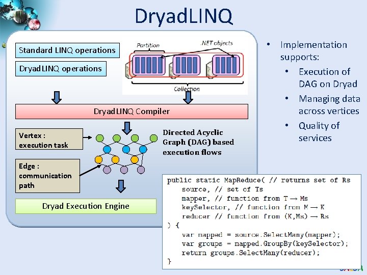
Dryad. LINQ Standard LINQ operations Dryad. LINQ Compiler Vertex : execution task Directed Acyclic Graph (DAG) based execution flows • Implementation supports: • Execution of DAG on Dryad • Managing data across vertices • Quality of services Edge : communication path Dryad Execution Engine SALSA

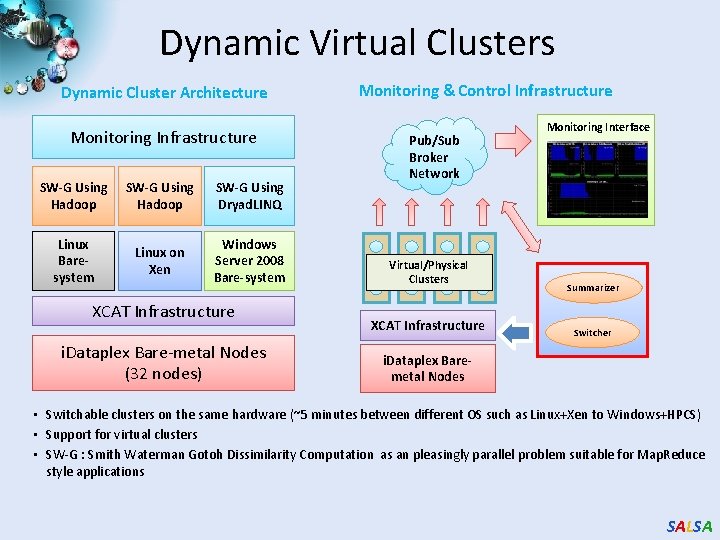
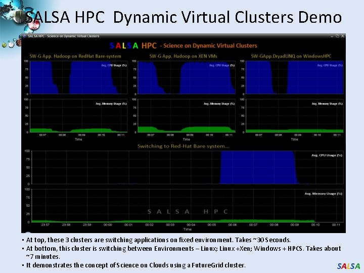
Dynamic Virtual Clusters Dynamic Cluster Architecture Monitoring Infrastructure SW-G Using Hadoop SW-G Using Dryad. LINQ Linux Baresystem Linux on Xen Windows Server 2008 Bare-system XCAT Infrastructure i. Dataplex Bare-metal Nodes (32 nodes) Monitoring & Control Infrastructure Pub/Sub Broker Network Virtual/Physical Clusters XCAT Infrastructure Monitoring Interface Summarizer Switcher i. Dataplex Baremetal Nodes • Switchable clusters on the same hardware (~5 minutes between different OS such as Linux+Xen to Windows+HPCS) • Support for virtual clusters • SW-G : Smith Waterman Gotoh Dissimilarity Computation as an pleasingly parallel problem suitable for Map. Reduce style applications SALSA

SALSA HPC Dynamic Virtual Clusters Demo • At top, these 3 clusters are switching applications on fixed environment. Takes ~30 Seconds. • At bottom, this cluster is switching between Environments – Linux; Linux +Xen; Windows + HPCS. Takes about ~7 minutes. • It demonstrates the concept of Science on Clouds using a Future. Grid cluster. SALSA

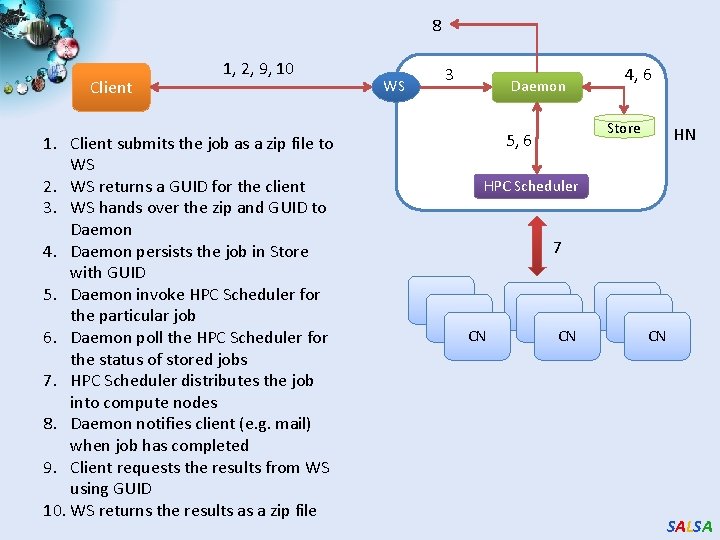
8 Client 1, 2, 9, 10 1. Client submits the job as a zip file to WS 2. WS returns a GUID for the client 3. WS hands over the zip and GUID to Daemon 4. Daemon persists the job in Store with GUID 5. Daemon invoke HPC Scheduler for the particular job 6. Daemon poll the HPC Scheduler for the status of stored jobs 7. HPC Scheduler distributes the job into compute nodes 8. Daemon notifies client (e. g. mail) when job has completed 9. Client requests the results from WS using GUID 10. WS returns the results as a zip file WS 3 Daemon 4, 6 Store 5, 6 HN HPC Scheduler 7 CN CN CN SALSA

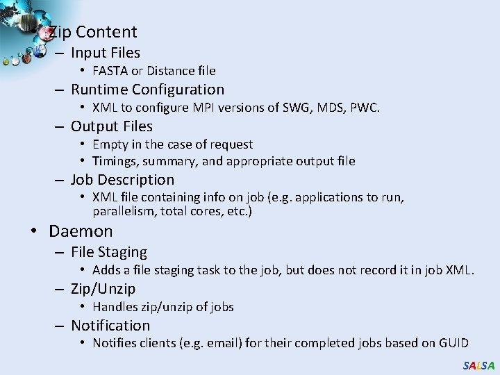
• Zip Content – Input Files • FASTA or Distance file – Runtime Configuration • XML to configure MPI versions of SWG, MDS, PWC. – Output Files • Empty in the case of request • Timings, summary, and appropriate output file – Job Description • XML file containing info on job (e. g. applications to run, parallelism, total cores, etc. ) • Daemon – File Staging • Adds a file staging task to the job, but does not record it in job XML. – Zip/Unzip • Handles zip/unzip of jobs – Notification • Notifies clients (e. g. email) for their completed jobs based on GUID SALSA

High Performance Dimension Reduction and Visualization • Need is pervasive – Large and high dimensional data are everywhere: biology, physics, Internet, … – Visualization can help data analysis • Visualization with high performance – Map high-dimensional data into low dimensions. – Need high performance for processing large data – Developing high performance visualization algorithms: MDS(Multi-dimensional Scaling), GTM(Generative Topographic Mapping), DA-MDS(Deterministic Annealing MDS), DA-GTM(Deterministic Annealing GTM), … SALSA

Dimension Reduction Algorithms • Multidimensional Scaling (MDS) [1] • Generative Topographic Mapping (GTM) [2] o Given the proximity information among points. o Optimization problem to find mapping in target dimension of the given data based on pairwise proximity information while minimize the objective function. o Objective functions: STRESS (1) or SSTRESS (2) o Find optimal K-representations for the given data (in 3 D), known as K-cluster problem (NP-hard) o Original algorithm use EM method for optimization o Deterministic Annealing algorithm can be used for finding a global solution o Objective functions is to maximize loglikelihood: o Only needs pairwise distances ij between original points (typically not Euclidean) o dij(X) is Euclidean distance between mapped (3 D) points [1] I. Borg and P. J. Groenen. Modern Multidimensional Scaling: Theory and Applications. Springer, New York, NY, U. S. A. , 2005. [2] C. Bishop, M. Svens´en, and C. Williams. GTM: The generative topographic mapping. Neural computation, 10(1): 215– 234, 1998. SALSA

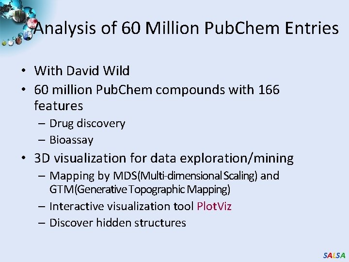
Analysis of 60 Million Pub. Chem Entries • With David Wild • 60 million Pub. Chem compounds with 166 features – Drug discovery – Bioassay • 3 D visualization for data exploration/mining – Mapping by MDS(Multi-dimensional Scaling) and GTM(Generative Topographic Mapping) – Interactive visualization tool Plot. Viz – Discover hidden structures SALSA

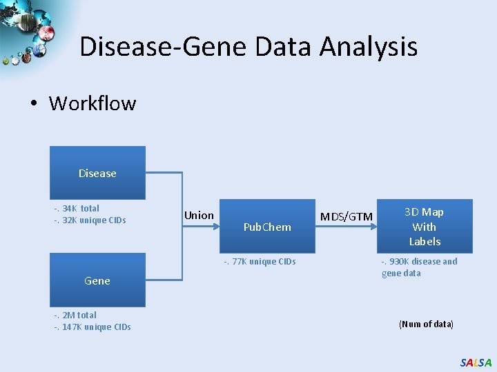
Disease-Gene Data Analysis • Workflow Disease -. 34 K total -. 32 K unique CIDs Union Pub. Chem -. 77 K unique CIDs Gene -. 2 M total -. 147 K unique CIDs MDS/GTM 3 D Map With Labels -. 930 K disease and gene data (Num of data) SALSA

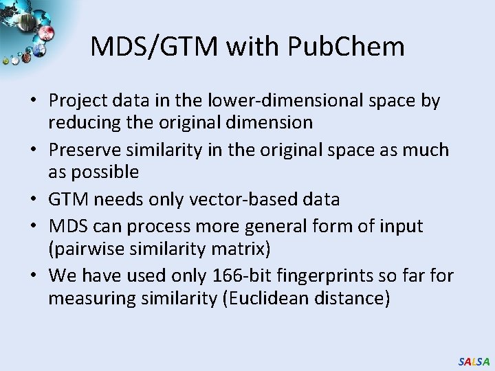
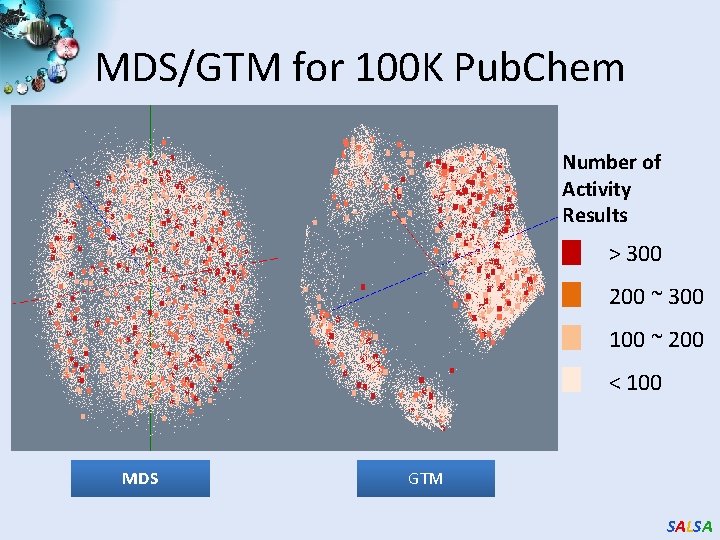
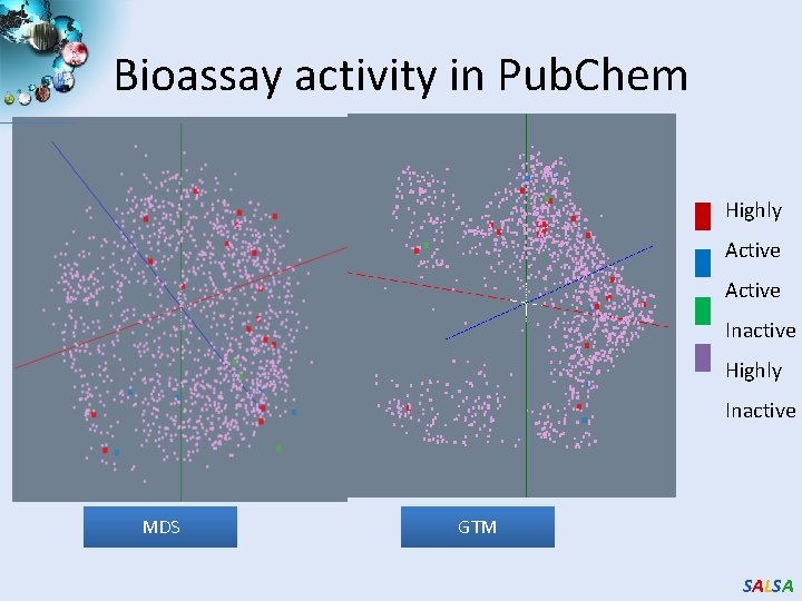
MDS/GTM with Pub. Chem • Project data in the lower-dimensional space by reducing the original dimension • Preserve similarity in the original space as much as possible • GTM needs only vector-based data • MDS can process more general form of input (pairwise similarity matrix) • We have used only 166 -bit fingerprints so far for measuring similarity (Euclidean distance) SALSA

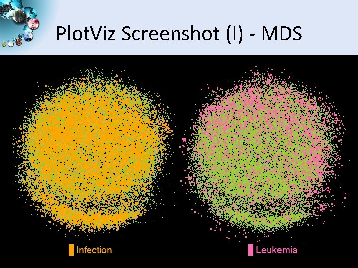
Plot. Viz Screenshot (I) - MDS SALSA

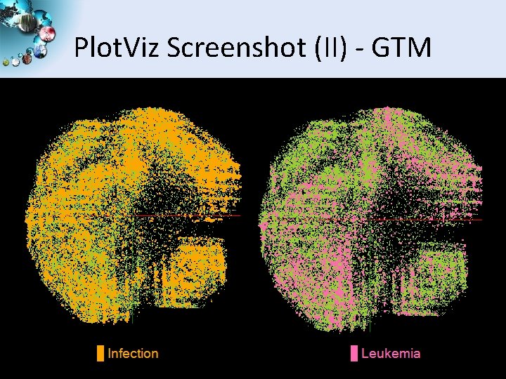
Plot. Viz Screenshot (II) - GTM SALSA

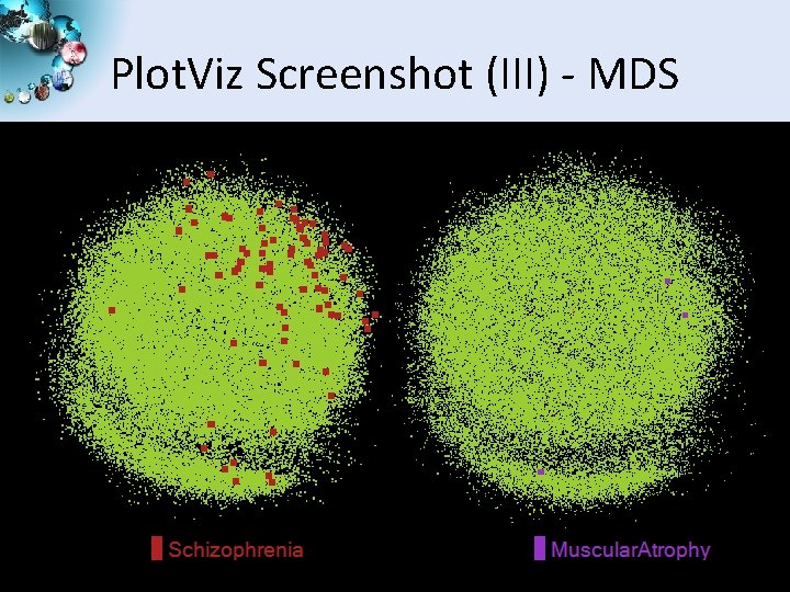
Plot. Viz Screenshot (III) - MDS SALSA

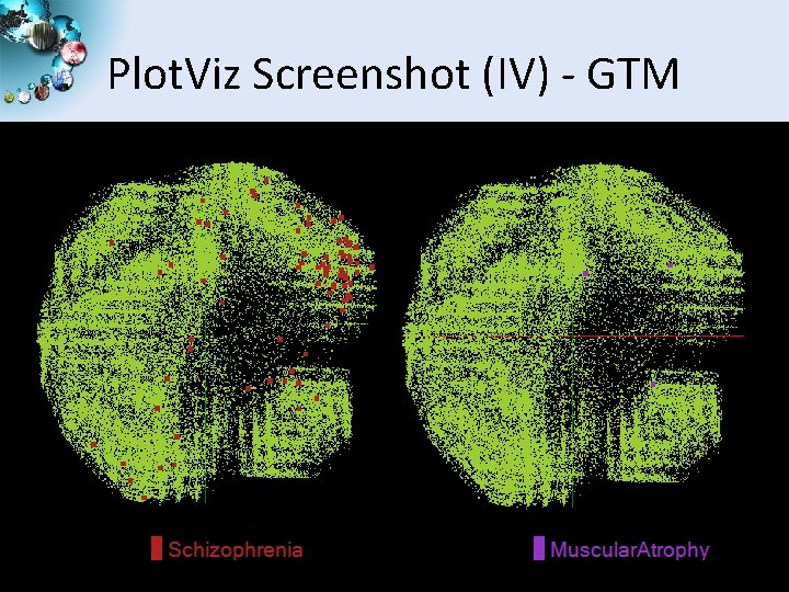
Plot. Viz Screenshot (IV) - GTM SALSA

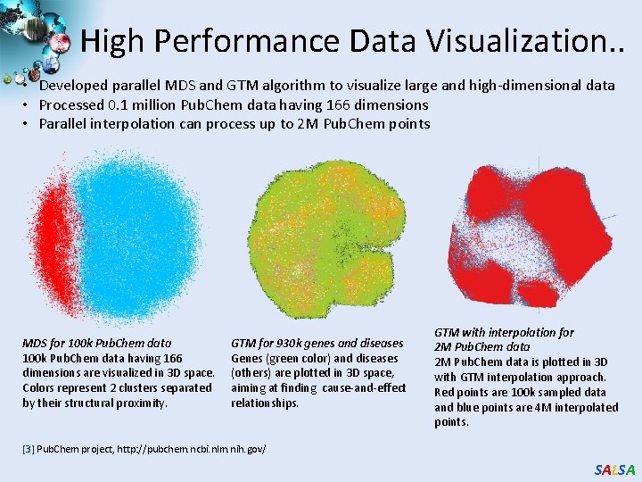
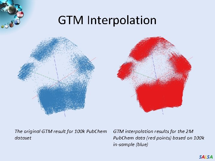
High Performance Data Visualization. . • Developed parallel MDS and GTM algorithm to visualize large and high-dimensional data • Processed 0. 1 million Pub. Chem data having 166 dimensions • Parallel interpolation can process up to 2 M Pub. Chem points MDS for 100 k Pub. Chem data having 166 dimensions are visualized in 3 D space. Colors represent 2 clusters separated by their structural proximity. GTM for 930 k genes and diseases Genes (green color) and diseases (others) are plotted in 3 D space, aiming at finding cause-and-effect relationships. GTM with interpolation for 2 M Pub. Chem data is plotted in 3 D with GTM interpolation approach. Red points are 100 k sampled data and blue points are 4 M interpolated points. [3] Pub. Chem project, http: //pubchem. ncbi. nlm. nih. gov/ SALSA

Dimension Reduction Algorithms • Multidimensional Scaling (MDS) [1] • Generative Topographic Mapping (GTM) [2] o Given the proximity information among points. o Optimization problem to find mapping in target dimension of the given data based on pairwise proximity information while minimize the objective function. o Objective functions: STRESS (1) or SSTRESS (2) o Find optimal K-representations for the given data (in 3 D), known as K-cluster problem (NP-hard) o Original algorithm use EM method for optimization o Deterministic Annealing algorithm can be used for finding a global solution o Objective functions is to maximize loglikelihood: o Only needs pairwise distances ij between original points (typically not Euclidean) o dij(X) is Euclidean distance between mapped (3 D) points [1] I. Borg and P. J. Groenen. Modern Multidimensional Scaling: Theory and Applications. Springer, New York, NY, U. S. A. , 2005. [2] C. Bishop, M. Svens´en, and C. Williams. GTM: The generative topographic mapping. Neural computation, 10(1): 215– 234, 1998. SALSA

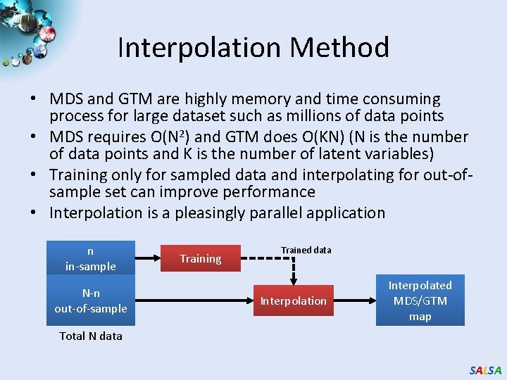
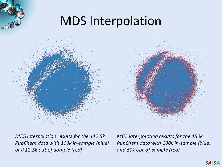
Interpolation Method • MDS and GTM are highly memory and time consuming process for large dataset such as millions of data points • MDS requires O(N 2) and GTM does O(KN) (N is the number of data points and K is the number of latent variables) • Training only for sampled data and interpolating for out-ofsample set can improve performance • Interpolation is a pleasingly parallel application n in-sample N-n out-of-sample Training Trained data Interpolation Interpolated MDS/GTM map Total N data SALSA

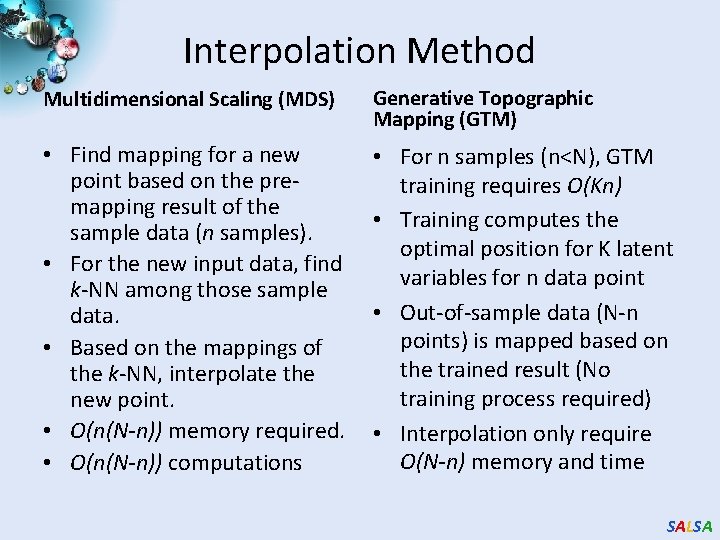
Interpolation Method Multidimensional Scaling (MDS) Generative Topographic Mapping (GTM) • Find mapping for a new point based on the premapping result of the sample data (n samples). • For the new input data, find k-NN among those sample data. • Based on the mappings of the k-NN, interpolate the new point. • O(n(N-n)) memory required. • O(n(N-n)) computations • For n samples (n<N), GTM training requires O(Kn) • Training computes the optimal position for K latent variables for n data point • Out-of-sample data (N-n points) is mapped based on the trained result (No training process required) • Interpolation only require O(N-n) memory and time SALSA

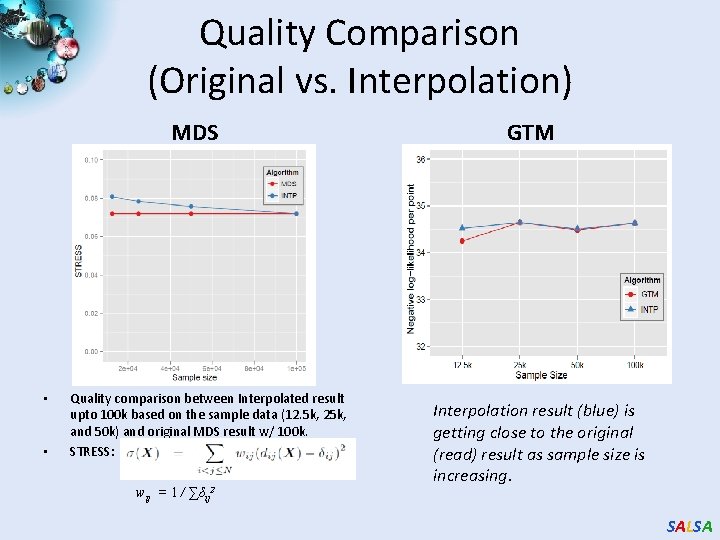
Quality Comparison (Original vs. Interpolation) MDS • • Quality comparison between Interpolated result upto 100 k based on the sample data (12. 5 k, 25 k, and 50 k) and original MDS result w/ 100 k. STRESS: wij = 1 / ∑δij 2 GTM Interpolation result (blue) is getting close to the original (read) result as sample size is increasing. SALSA

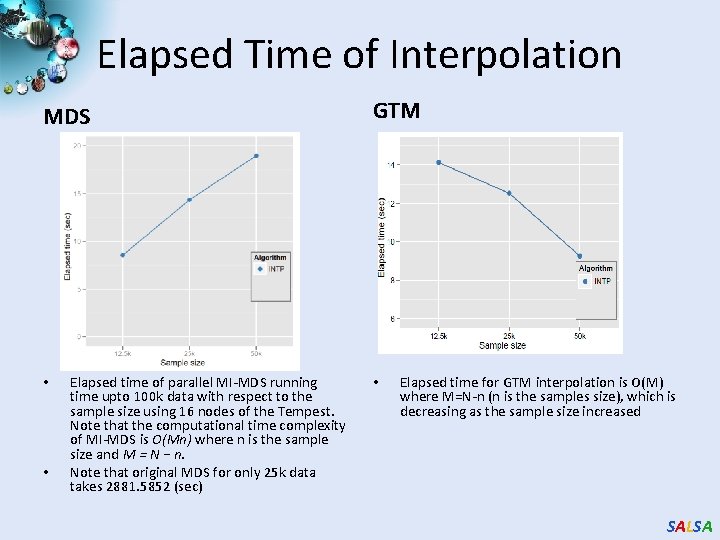
Elapsed Time of Interpolation MDS • • Elapsed time of parallel MI-MDS running time upto 100 k data with respect to the sample size using 16 nodes of the Tempest. Note that the computational time complexity of MI-MDS is O(Mn) where n is the sample size and M = N − n. Note that original MDS for only 25 k data takes 2881. 5852 (sec) GTM • Elapsed time for GTM interpolation is O(M) where M=N-n (n is the samples size), which is decreasing as the sample size increased SALSA

MDS Interpolation MDS interpolation results for the 112. 5 k Pub. Chem data with 100 k in-sample (blue) and 12. 5 k out-of-sample (red) MDS interpolation results for the 150 k Pub. Chem data with 100 k in-sample (blue) and 50 k out-of-sample (red) SALSA

GTM Interpolation The original GTM result for 100 k Pub. Chem dataset GTM interpolation results for the 2 M Pub. Chem data (red points) based on 100 k in-sample (blue) SALSA

MDS/GTM for 100 K Pub. Chem Number of Activity Results > 300 200 ~ 300 100 ~ 200 < 100 MDS GTM SALSA

Bioassay activity in Pub. Chem Highly Active Inactive Highly Inactive MDS GTM SALSA

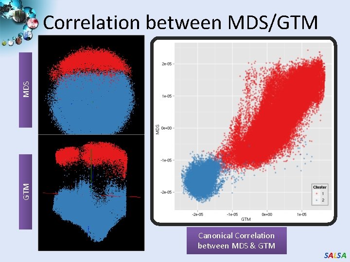
GTM MDS Correlation between MDS/GTM Canonical Correlation between MDS & GTM SALSA

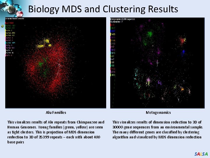
Biology MDS and Clustering Results Alu Families Metagenomics This visualizes results of Alu repeats from Chimpanzee and Human Genomes. Young families (green, yellow) are seen as tight clusters. This is projection of MDS dimension reduction to 3 D of 35399 repeats – each with about 400 base pairs This visualizes results of dimension reduction to 3 D of 30000 gene sequences from an environmental sample. The many different genes are classified by clustering algorithm and visualized by MDS dimension reduction SALSA

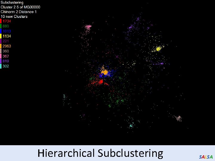
Hierarchical Subclustering SALSA

Applications using Dryad & Dryad. LINQ (1) CAP 3 [1] - Expressed Sequence Tag assembly to re-construct full-length m. RNA Time to process 1280 files each with ~375 sequences Input files (FASTA) CAP 3 Output files CAP 3 Average Time (Seconds) 700 600 500 Hadoop Dryad. LINQ 400 300 200 100 0 • Perform using Dryad. LINQ and Apache Hadoop implementations • Single “Select” operation in Dryad. LINQ • “Map only” operation in Hadoop [4] X. Huang, A. Madan, “CAP 3: A DNA Sequence Assembly Program, ” Genome Research, vol. 9, no. 9, pp. 868 -877, 1999. SALSA

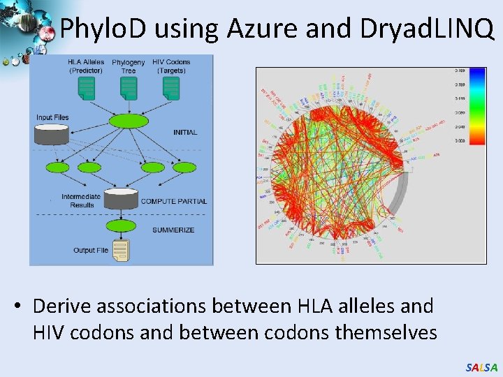
Applications using Dryad & Dryad. LINQ (2) Phylo. D [2] project from Microsoft Research • Output of Phylo. D shows the associations • Derive associations between HLA alleles and HIV codons and between codons themselves 2000 1800 1600 1400 1200 1000 800 600 400 200 0 Avg. Time per Pair 0 50000 100000 Number of HLA&HIV Pairs 50 45 40 35 30 25 20 15 10 5 0 150000 Avg. Time to Calculate a Pair (milliseconds) Avg. time on 48 CPU cores (Seconds) Scalability of Dryad. LINQ Phylo. D Application [5] Microsoft Computational Biology Web Tools, http: //research. microsoft. com/en-us/um/redmond/projects/MSComp. Bio/ SALSA

All-Pairs[3] Using Dryad. LINQ 125 million distances 4 hours & 46 minutes 20000 15000 Dryad. LINQ MPI 10000 5000 Calculate Pairwise Distances (Smith Waterman Gotoh) • • 0 35339 50000 Calculate pairwise distances for a collection of genes (used for clustering, MDS) Fine grained tasks in MPI Coarse grained tasks in Dryad. LINQ Performed on 768 cores (Tempest Cluster) [5] Moretti, C. , Bui, H. , Hollingsworth, K. , Rich, B. , Flynn, P. , & Thain, D. (2009). All-Pairs: An Abstraction for Data Intensive Computing on Campus Grids. IEEE Transactions on Parallel and Distributed Systems , 21 -36. SALSA

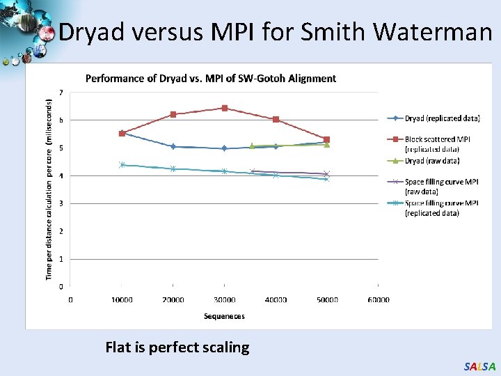
Dryad versus MPI for Smith Waterman Flat is perfect scaling SALSA

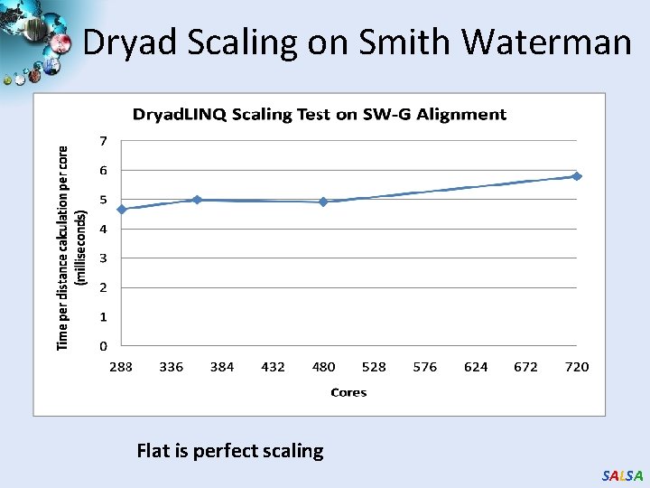
Dryad Scaling on Smith Waterman Flat is perfect scaling SALSA

Dryad for Inhomogeneous Data Calculation Time per Pair [A, B] α Length A * Length B Total Time (ms) Mean Length 400 Computation Sequence Length Standard Deviation Flat is perfect scaling – measured on Tempest SALSA

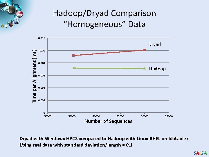
Hadoop/Dryad Comparison “Homogeneous” Data 0, 012 Time per Alignment (ms) Dryad 0, 01 0, 008 Hadoop 0, 006 0, 004 0, 002 0 30000 35000 40000 45000 Number of Sequences 50000 55000 Dryad with Windows HPCS compared to Hadoop with Linux RHEL on Idataplex Using real data with standard deviation/length = 0. 1 SALSA

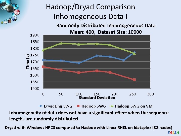
Time (s) Hadoop/Dryad Comparison Inhomogeneous Data I 1900 1850 1800 1750 1700 1650 1600 1550 1500 Randomly Distributed Inhomogeneous Data Mean: 400, Dataset Size: 10000 0 50 Dryad. Linq SWG 100 150 200 Standard Deviation Hadoop SWG 250 300 Hadoop SWG on VM Inhomogeneity of data does not have a significant effect when the sequence lengths are randomly distributed Dryad with Windows HPCS compared to Hadoop with Linux RHEL on Idataplex (32 nodes) SALSA

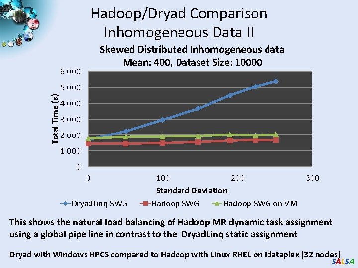
Hadoop/Dryad Comparison Inhomogeneous Data II Skewed Distributed Inhomogeneous data Mean: 400, Dataset Size: 10000 6 000 Total Time (s) 5 000 4 000 3 000 2 000 1 000 0 0 Dryad. Linq SWG 100 200 Standard Deviation Hadoop SWG 300 Hadoop SWG on VM This shows the natural load balancing of Hadoop MR dynamic task assignment using a global pipe line in contrast to the Dryad. Linq static assignment Dryad with Windows HPCS compared to Hadoop with Linux RHEL on Idataplex (32 nodes) SALSA

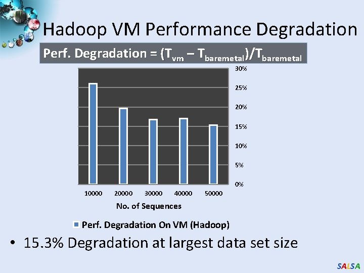
Hadoop VM Performance Degradation Perf. Degradation = (Tvm – Tbaremetal)/Tbaremetal 30% 25% 20% 15% 10% 5% 0% 10000 20000 30000 40000 50000 No. of Sequences Perf. Degradation On VM (Hadoop) • 15. 3% Degradation at largest data set size SALSA

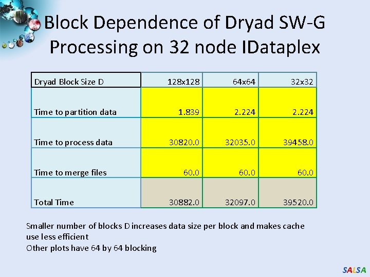
Block Dependence of Dryad SW-G Processing on 32 node IDataplex Dryad Block Size D Time to partition data Time to process data Time to merge files Total Time 128 x 128 64 x 64 32 x 32 1. 839 2. 224 30820. 0 32035. 0 39458. 0 60. 0 30882. 0 32097. 0 39520. 0 Smaller number of blocks D increases data size per block and makes cache use less efficient Other plots have 64 by 64 blocking SALSA

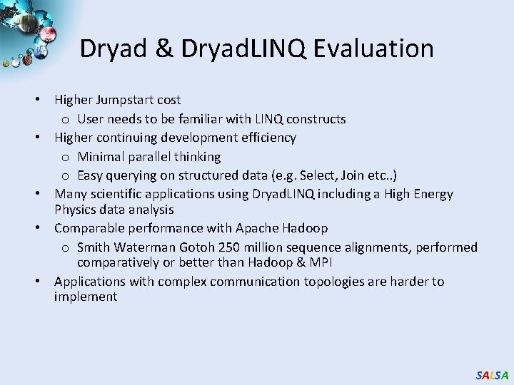
Dryad & Dryad. LINQ Evaluation • Higher Jumpstart cost o User needs to be familiar with LINQ constructs • Higher continuing development efficiency o Minimal parallel thinking o Easy querying on structured data (e. g. Select, Join etc. . ) • Many scientific applications using Dryad. LINQ including a High Energy Physics data analysis • Comparable performance with Apache Hadoop o Smith Waterman Gotoh 250 million sequence alignments, performed comparatively or better than Hadoop & MPI • Applications with complex communication topologies are harder to implement SALSA

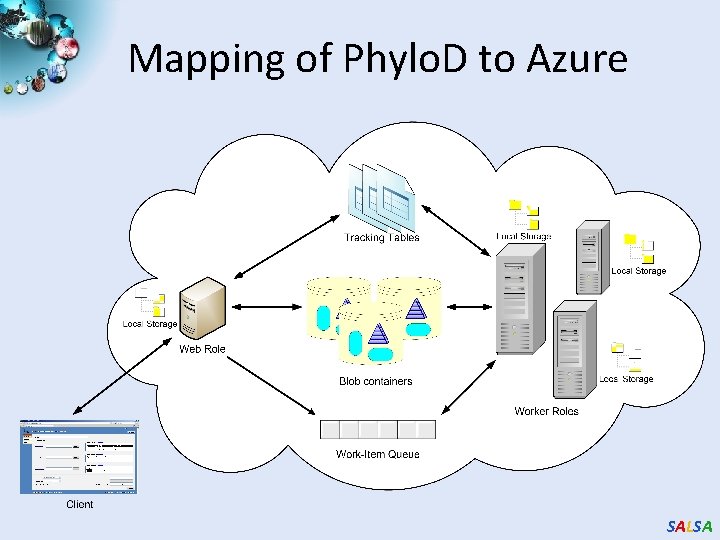
Phylo. D using Azure and Dryad. LINQ • Derive associations between HLA alleles and HIV codons and between codons themselves SALSA

Mapping of Phylo. D to Azure SALSA

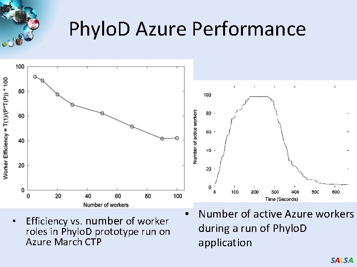
Phylo. D Azure Performance • Efficiency vs. number of worker roles in Phylo. D prototype run on Azure March CTP • Number of active Azure workers during a run of Phylo. D application SALSA

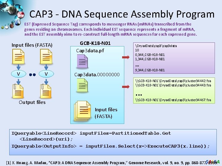
CAP 3 - DNA Sequence Assembly Program EST (Expressed Sequence Tag) corresponds to messenger RNAs (m. RNAs) transcribed from the genes residing on chromosomes. Each individual EST sequence represents a fragment of m. RNA, and the EST assembly aims to re-construct full-length m. RNA sequences for each expressed gene. Input files (FASTA) GCB-K 18 -N 01 Cap 3 data. pf Dryad. Datacap 3 data 10 0, 344, CGB-K 18 -N 01 1, 344, CGB-K 18 -N 01 … V V Cap 3 data. 0000 9, 344, CGB-K 18 -N 01 \GCB-K 18 -N 01Dryad. Datacap 3cluster 34442. fsa \GCB-K 18 -N 01Dryad. Datacap 3cluster 34443. fsa . . . \GCB-K 18 -N 01Dryad. Datacap 3cluster 34467. fsa Output files Input files (FASTA) IQueryable<Line. Record> input. Files=Partitioned. Table. Get <Line. Record>(uri); IQueryable<Output. Info> = input. Files. Select(x=>Execute. CAP 3(x. line)); [1] X. Huang, A. Madan, “CAP 3: A DNA Sequence Assembly Program, ” Genome Research, vol. 9, no. 9, pp. 868 -877, SALSA 1999.

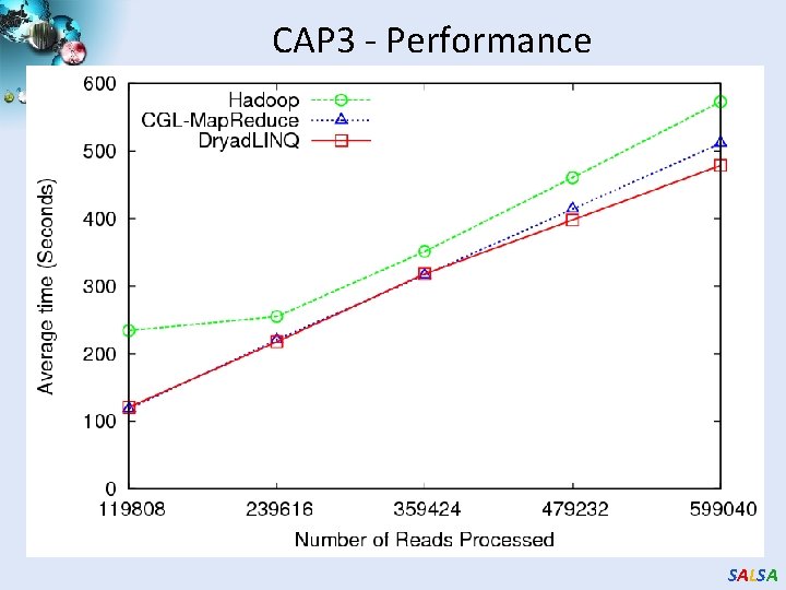
CAP 3 - Performance SALSA

Application Classes Old classification of Parallel software/hardware in terms of 5 (becoming 6) “Application architecture” Structures) 1 Synchronous Lockstep Operation as in SIMD architectures 2 Loosely Synchronous Iterative Compute-Communication stages with independent compute (map) operations for each CPU. Heart of most MPI jobs MPP 3 Asynchronous Compute Chess; Combinatorial Search often supported by dynamic threads MPP 4 Pleasingly Parallel Each component independent – in 1988, Fox estimated at 20% of total number of applications Grids 5 Metaproblems Coarse grain (asynchronous) combinations of classes 1)4). The preserve of workflow. Grids 6 Map. Reduce++ It describes file(database) to file(database) operations which has subcategories including. 1) Pleasingly Parallel Map Only 2) Map followed by reductions 3) Iterative “Map followed by reductions” – Extension of Current Technologies that supports much linear algebra and datamining Clouds Hadoop/ Dryad Twister SALSA

Applications & Different Interconnection Patterns Map Only Input map Output Classic Map. Reduce Input map Ite rative Reductions Map. Reduce++ Input map Loosely Synchronous iterations Pij reduce CAP 3 Analysis Document conversion (PDF -> HTML) Brute force searches in cryptography Parametric sweeps High Energy Physics (HEP) Histograms SWG gene alignment Distributed search Distributed sorting Information retrieval Expectation maximization algorithms Clustering Linear Algebra Many MPI scientific applications utilizing wide variety of communication constructs including local interactions - CAP 3 Gene Assembly - Polar. Grid Matlab data analysis - Information Retrieval HEP Data Analysis - Calculation of Pairwise Distances for ALU Sequences - Kmeans - Deterministic Annealing Clustering - Multidimensional Scaling MDS - Solving Differential Equations and - particle dynamics with short range forces Domain of Map. Reduce and Iterative Extensions MPI SALSA

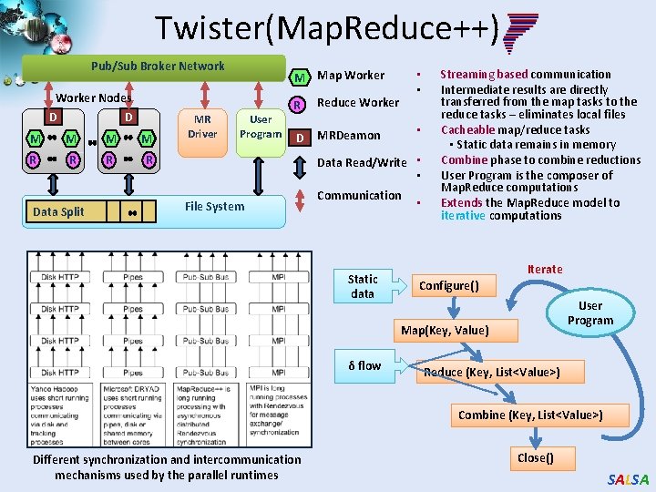
Twister(Map. Reduce++) Pub/Sub Broker Network Worker Nodes D D M M R R Data Split MR Driver • • M Map Worker User Program R Reduce Worker D MRDeamon • Data Read/Write • • File System Communication Static data • Streaming based communication Intermediate results are directly transferred from the map tasks to the reduce tasks – eliminates local files Cacheable map/reduce tasks • Static data remains in memory Combine phase to combine reductions User Program is the composer of Map. Reduce computations Extends the Map. Reduce model to iterative computations Iterate Configure() User Program Map(Key, Value) δ flow Reduce (Key, List<Value>) Combine (Key, List<Value>) Different synchronization and intercommunication mechanisms used by the parallel runtimes Close() SALSA

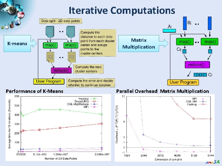
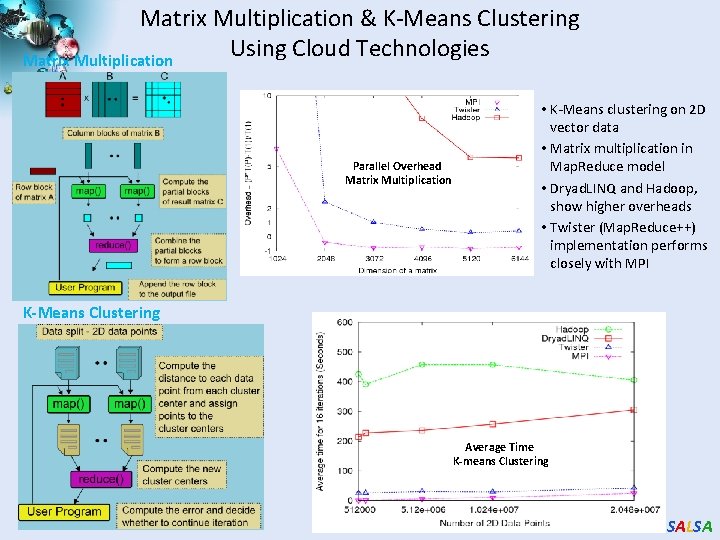
Iterative Computations K-means Performance of K-Means Matrix Multiplication Parallel Overhead Matrix Multiplication SALSA

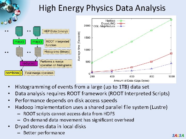
High Energy Physics Data Analysis • • Histogramming of events from a large (up to 1 TB) data set Data analysis requires ROOT framework (ROOT Interpreted Scripts) Performance depends on disk access speeds Hadoop implementation uses a shared parallel file system (Lustre) – ROOT scripts cannot access data from HDFS – On demand data movement has significant overhead • Dryad stores data in local disks – Better performance SALSA

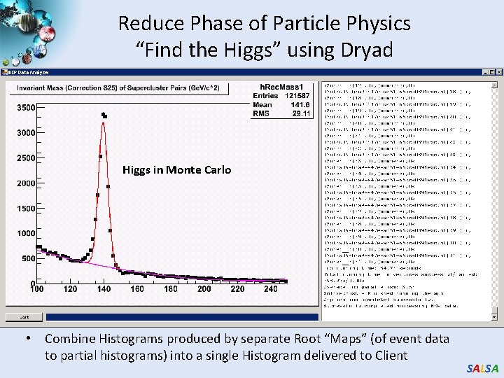
Reduce Phase of Particle Physics “Find the Higgs” using Dryad Higgs in Monte Carlo • Combine Histograms produced by separate Root “Maps” (of event data to partial histograms) into a single Histogram delivered to Client SALSA

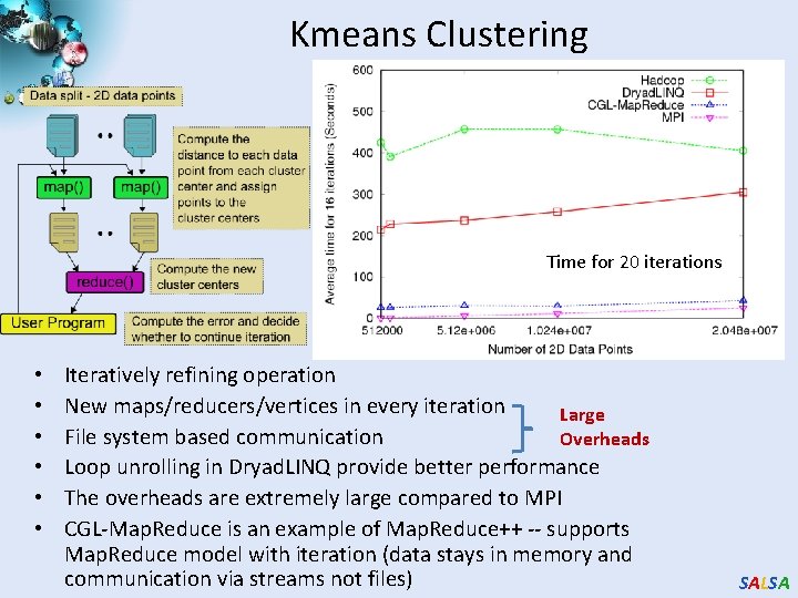
Kmeans Clustering Time for 20 iterations • • • Iteratively refining operation New maps/reducers/vertices in every iteration Large File system based communication Overheads Loop unrolling in Dryad. LINQ provide better performance The overheads are extremely large compared to MPI CGL-Map. Reduce is an example of Map. Reduce++ -- supports Map. Reduce model with iteration (data stays in memory and communication via streams not files) SALSA

Matrix Multiplication & K-Means Clustering Using Cloud Technologies Matrix Multiplication Parallel Overhead Matrix Multiplication • K-Means clustering on 2 D vector data • Matrix multiplication in Map. Reduce model • Dryad. LINQ and Hadoop, show higher overheads • Twister (Map. Reduce++) implementation performs closely with MPI K-Means Clustering Average Time K-means Clustering SALSA

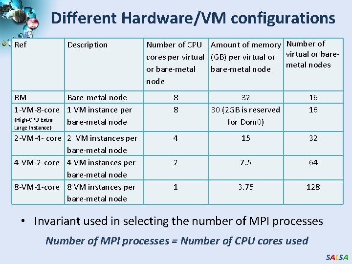
Different Hardware/VM configurations Ref Description Number of CPU Amount of memory Number of cores per virtual (GB) per virtual or baremetal nodes or bare-metal node BM Bare-metal node 1 -VM-8 -core 1 VM instance per (High-CPU Extra bare-metal node 8 8 32 30 (2 GB is reserved for Dom 0) 16 16 2 -VM-4 - core 2 VM instances per bare-metal node 4 -VM-2 -core 4 VM instances per bare-metal node 8 -VM-1 -core 8 VM instances per bare-metal node 4 15 32 2 7. 5 64 1 3. 75 128 Large Instance) • Invariant used in selecting the number of MPI processes Number of MPI processes = Number of CPU cores used SALSA

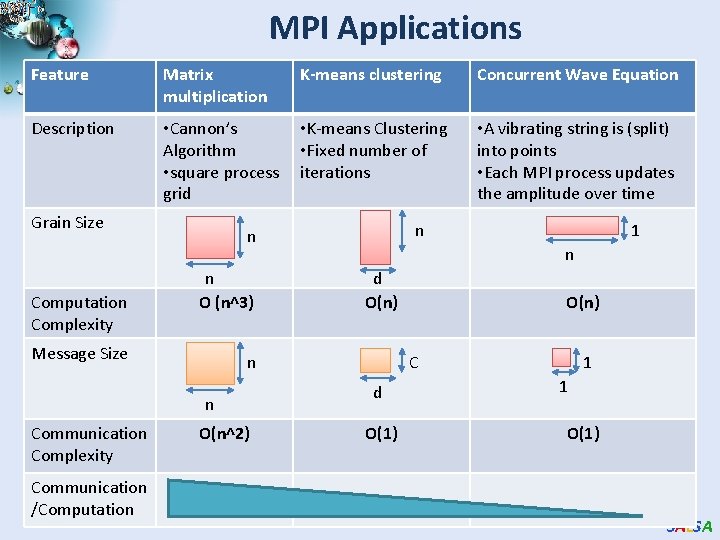
MPI Applications Feature Matrix multiplication K-means clustering Concurrent Wave Equation Description • Cannon’s Algorithm • square process grid • K-means Clustering • Fixed number of iterations • A vibrating string is (split) into points • Each MPI process updates the amplitude over time Grain Size Computation Complexity n O (n^3) Message Size Communication /Computation O(n^2) 1 n d O(n) n n Communication Complexity n n O(n) C d O(1) 1 1 O(1) SALSA

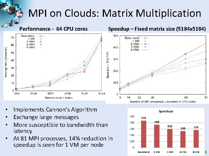
MPI on Clouds: Matrix Multiplication Performance - 64 CPU cores Speedup – Fixed matrix size (5184 x 5184) • Implements Cannon’s Algorithm • Exchange large messages • More susceptible to bandwidth than latency • At 81 MPI processes, 14% reduction in speedup is seen for 1 VM per node SALSA

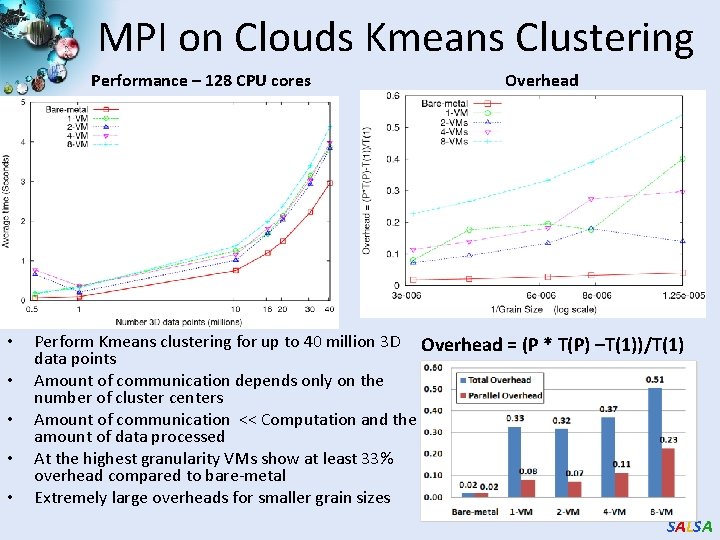
MPI on Clouds Kmeans Clustering Performance – 128 CPU cores • • • Overhead Perform Kmeans clustering for up to 40 million 3 D Overhead = (P * T(P) –T(1))/T(1) data points Amount of communication depends only on the number of cluster centers Amount of communication << Computation and the amount of data processed At the highest granularity VMs show at least 33% overhead compared to bare-metal Extremely large overheads for smaller grain sizes SALSA

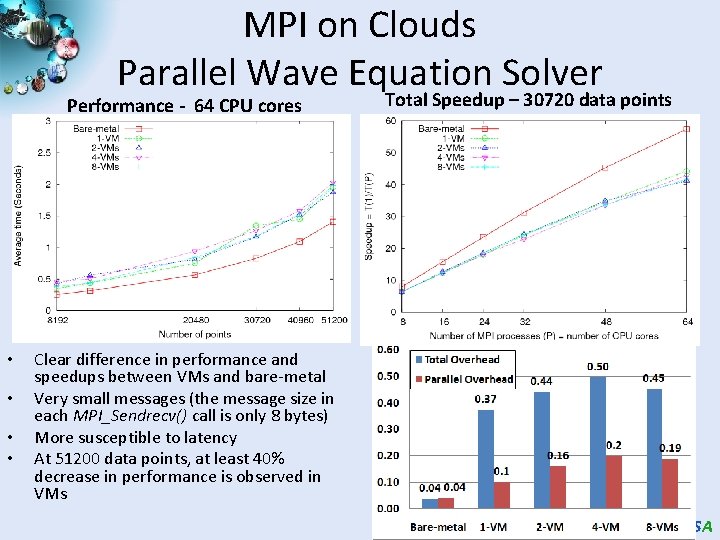
MPI on Clouds Parallel Wave Equation Solver Performance - 64 CPU cores • • Total Speedup – 30720 data points Clear difference in performance and speedups between VMs and bare-metal Very small messages (the message size in each MPI_Sendrecv() call is only 8 bytes) More susceptible to latency At 51200 data points, at least 40% decrease in performance is observed in VMs SALSA

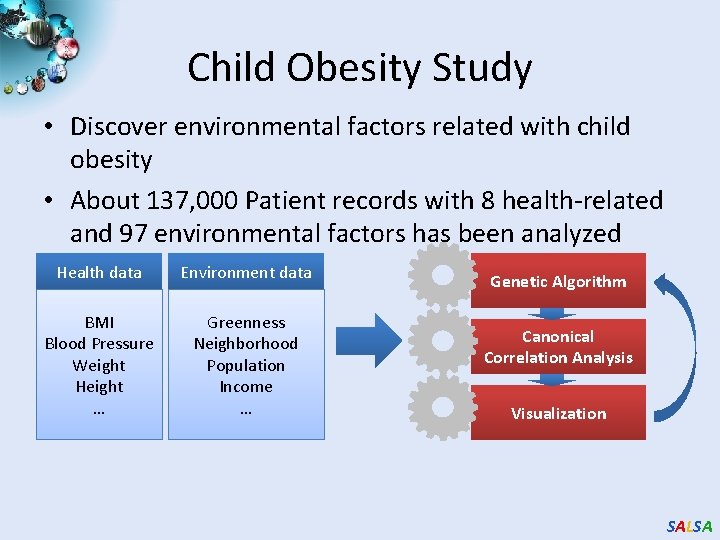
Child Obesity Study • Discover environmental factors related with child obesity • About 137, 000 Patient records with 8 health-related and 97 environmental factors has been analyzed Health data Environment data BMI Blood Pressure Weight Height … Greenness Neighborhood Population Income … Genetic Algorithm Canonical Correlation Analysis Visualization SALSA

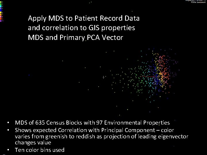
Apply MDS to Patient Record Data and correlation to GIS properties MDS and Primary PCA Vector • MDS of 635 Census Blocks with 97 Environmental Properties • Shows expected Correlation with Principal Component – color varies from greenish to reddish as projection of leading eigenvector changes value • Ten color bins used SALSA

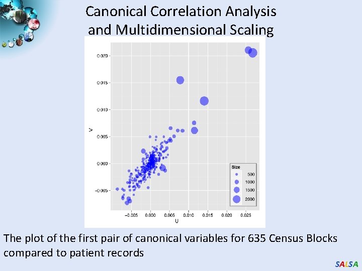
Canonical Correlation Analysis and Multidimensional Scaling The plot of the first pair of canonical variables for 635 Census Blocks compared to patient records SALSA

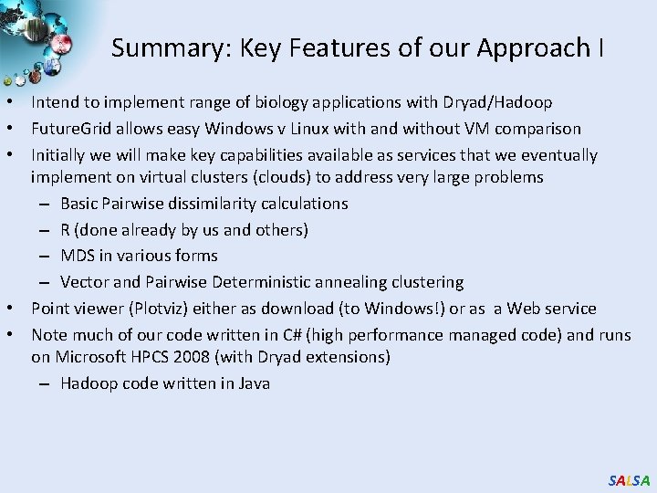
Summary: Key Features of our Approach I • Intend to implement range of biology applications with Dryad/Hadoop • Future. Grid allows easy Windows v Linux with and without VM comparison • Initially we will make key capabilities available as services that we eventually implement on virtual clusters (clouds) to address very large problems – Basic Pairwise dissimilarity calculations – R (done already by us and others) – MDS in various forms – Vector and Pairwise Deterministic annealing clustering • Point viewer (Plotviz) either as download (to Windows!) or as a Web service • Note much of our code written in C# (high performance managed code) and runs on Microsoft HPCS 2008 (with Dryad extensions) – Hadoop code written in Java SALSA

Summary: Key Features of our Approach II • Dryad/Hadoop/Azure promising for Biology computations • Dynamic Virtual Clusters allow one to switch between different modes • Overhead of VM’s on Hadoop (15%) acceptable • Inhomogeneous problems currently favors Hadoop over Dryad • Map. Reduce++ allows iterative problems (classic linear algebra/datamining) to use Map. Reduce model efficiently – Prototype Twister released SALSA

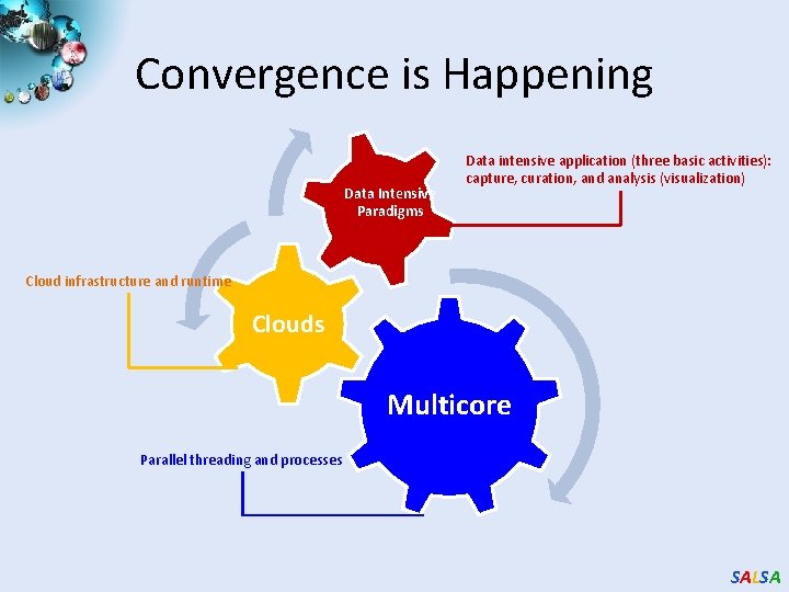
Convergence is Happening Data Intensive Paradigms Data intensive application (three basic activities): capture, curation, and analysis (visualization) Cloud infrastructure and runtime Clouds Multicore Parallel threading and processes SALSA

DNA Sequencing Pipeline Illumina/Solexa Roche/454 Life Sciences Applied Biosystems/SOLi. D Internet ~300 million base pairs per day leading to ~3000 sequences per day per instrument ? 500 instruments at ~0. 5 M$ each Read Alignment Pairwise clustering FASTA File N Sequences Blocking Form block Pairings Sequence alignment Dissimilarity Matrix MPI Visualization Plotviz N(N-1)/2 values MDS Map. Reduce SALSA

Future Work • The support for handling large data sets, the concept of moving computation to data, and the better quality of services provided by cloud technologies, make data analysis feasible on an unprecedented scale for assisting new scientific discovery. To facilitate the sharing of the latest research on novel "computational thinking", SALSA