Chapter 7 FIR Digital Filter Design Introduce In

Chapter 7 FIR Digital Filter Design

Introduce ¡ ¡ ¡ In this chapter, we consider the FIR digital filter design problem. Unlike the IIR digital filter design problem, it is always possible to design FIR digital filters with exact linear-phase. In the case of FIR digital filter design, the stability is not a design issue as the transfer function is a polynomial in z-1.

Introduce ¡ First, we describe a popular approach to the design of FIR digital filters with linearphase. ¡ We then consider the computer-aided design of linear-phase FIR digital filters. ¡ To this end, we restrict our discussion to the use of MATLAB in determining the transfer functions.

Advantages ¡ FIR digital filter is always guaranteed stable. ¡ It is always possible to design FIR digital filters with exact linear-phase.

Disadvantages ¡ The order of the FIR transfer function is usually much higher than that of an IIR transfer function meeting the same frequency response specification.

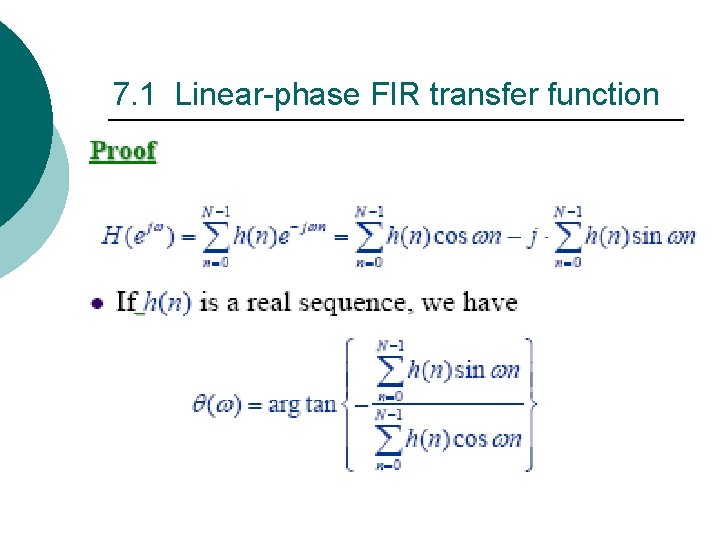
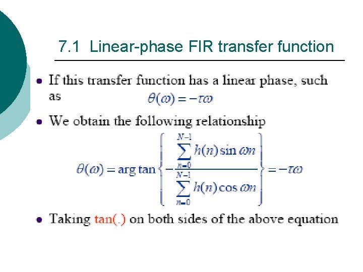
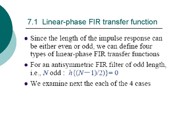
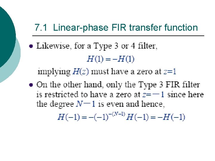
7. 1 Linear-phase FIR transfer function In the previous section, we pointed out why it is important to have a transfer function with a linear-phase property. In this section, we develop the forms of a linear-phase FIR transfer function H(z) with real impulse response h(n).

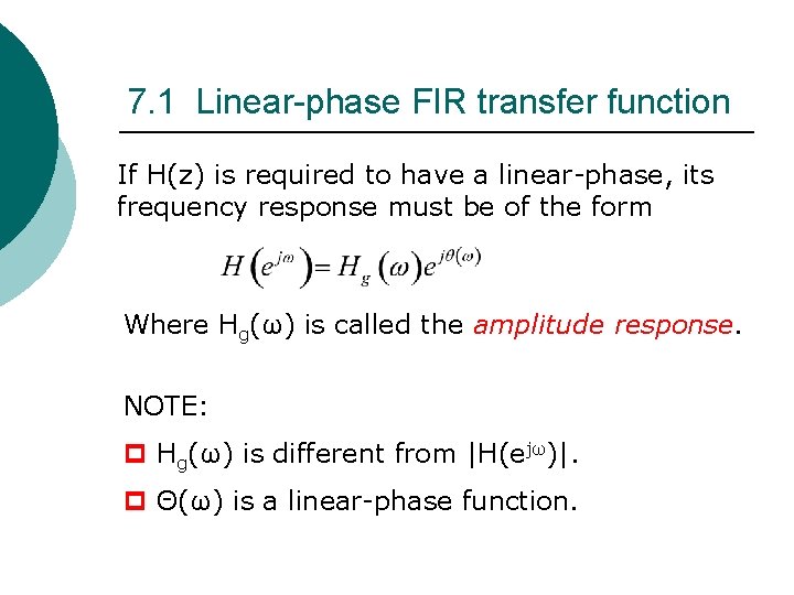
7. 1 Linear-phase FIR transfer function If H(z) is required to have a linear-phase, its frequency response must be of the form Where Hg(ω) is called the amplitude response. NOTE: p Hg(ω) is different from |H(ejω)|. p Θ(ω) is a linear-phase function.

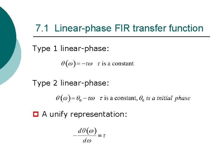
7. 1 Linear-phase FIR transfer function Type 1 linear-phase: Type 2 linear-phase: p A unify representation:

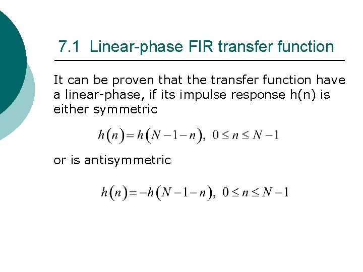
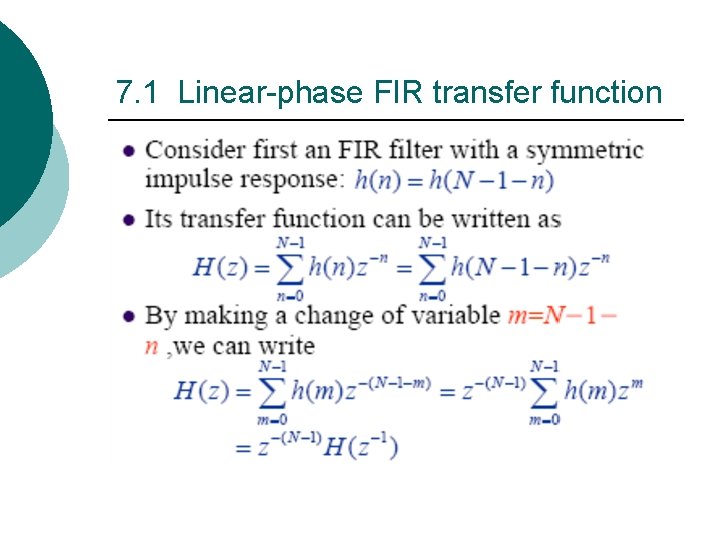
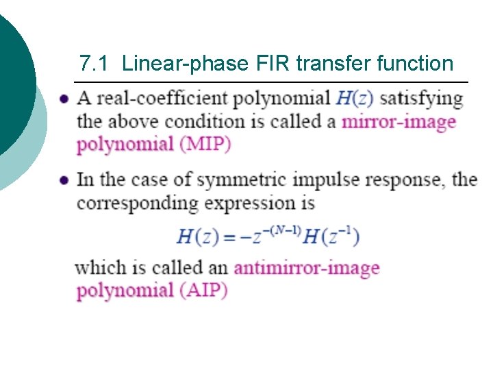
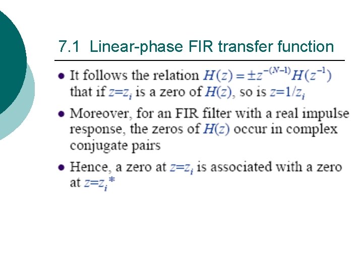
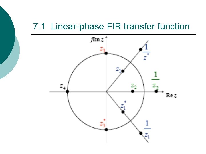
7. 1 Linear-phase FIR transfer function It can be proven that the transfer function have a linear-phase, if its impulse response h(n) is either symmetric or is antisymmetric

7. 1 Linear-phase FIR transfer function

7. 1 Linear-phase FIR transfer function

7. 1 Linear-phase FIR transfer function

7. 1 Linear-phase FIR transfer function

7. 1 Linear-phase FIR transfer function

7. 1 Linear-phase FIR transfer function

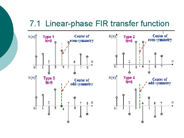
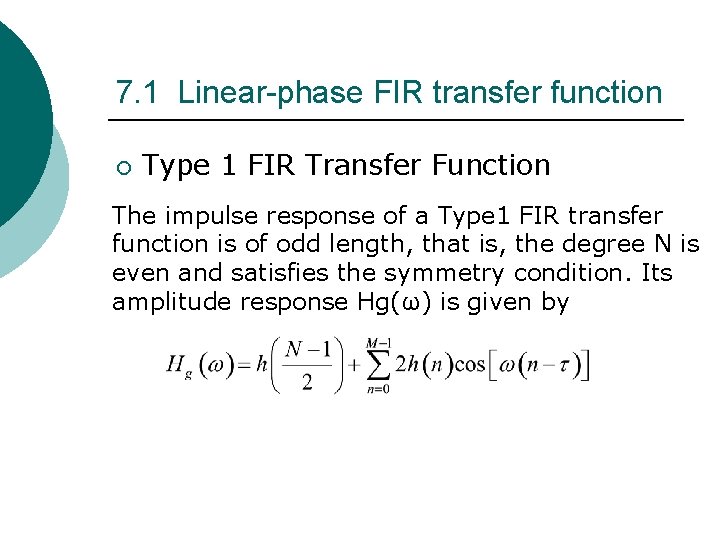
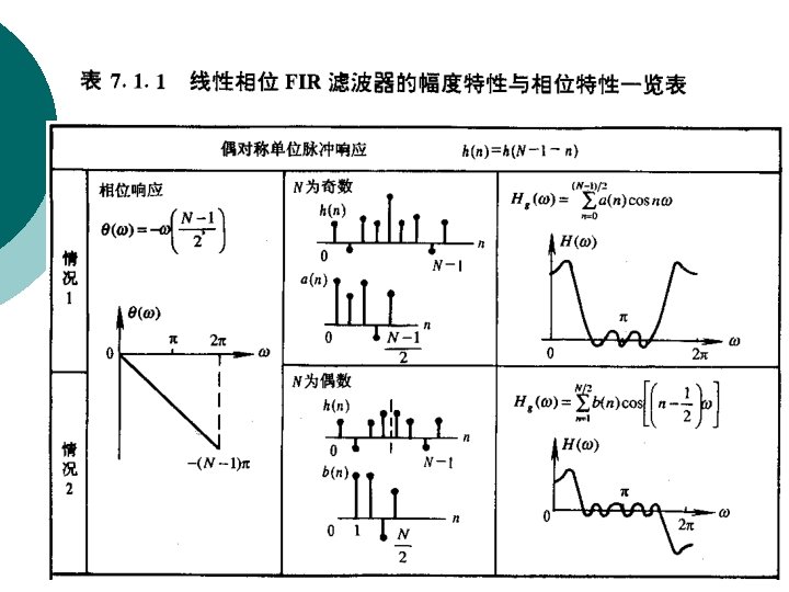
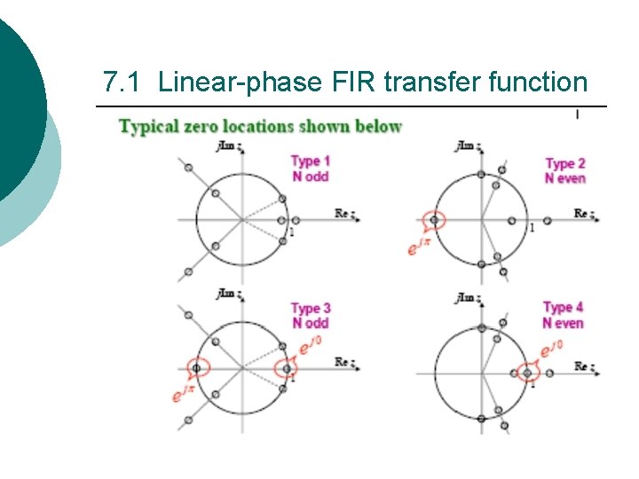
7. 1 Linear-phase FIR transfer function ¡ Type 1 FIR Transfer Function The impulse response of a Type 1 FIR transfer function is of odd length, that is, the degree N is even and satisfies the symmetry condition. Its amplitude response Hg(ω) is given by

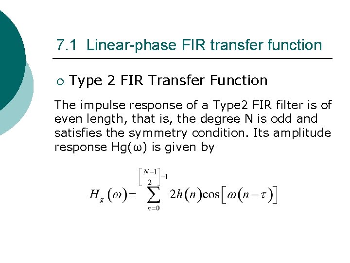
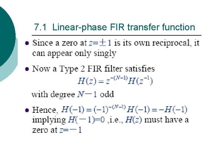
7. 1 Linear-phase FIR transfer function ¡ Type 2 FIR Transfer Function The impulse response of a Type 2 FIR filter is of even length, that is, the degree N is odd and satisfies the symmetry condition. Its amplitude response Hg(ω) is given by

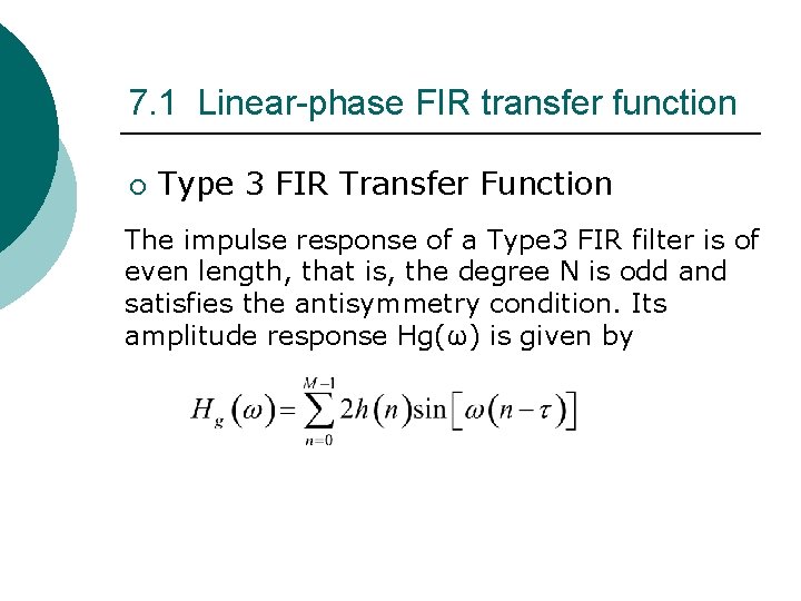
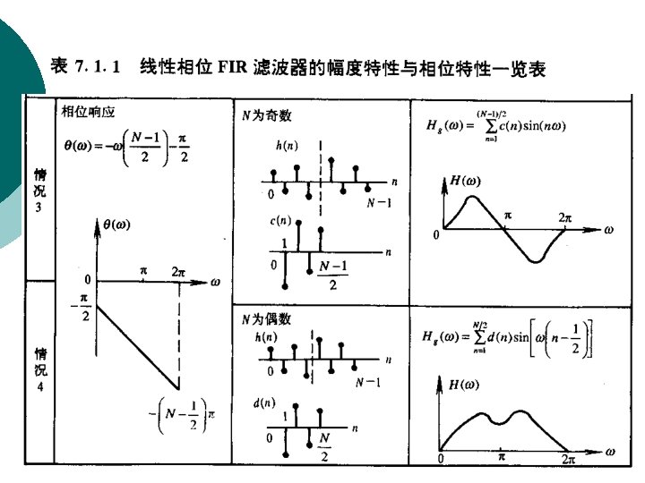
7. 1 Linear-phase FIR transfer function ¡ Type 3 FIR Transfer Function The impulse response of a Type 3 FIR filter is of even length, that is, the degree N is odd and satisfies the antisymmetry condition. Its amplitude response Hg(ω) is given by

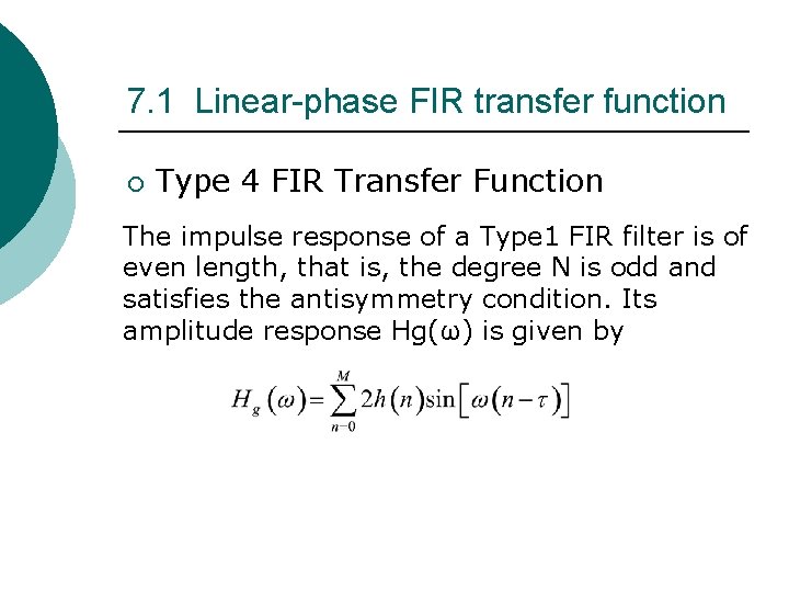
7. 1 Linear-phase FIR transfer function ¡ Type 4 FIR Transfer Function The impulse response of a Type 1 FIR filter is of even length, that is, the degree N is odd and satisfies the antisymmetry condition. Its amplitude response Hg(ω) is given by

7. 1 Linear-phase FIR transfer function

7. 1 Linear-phase FIR transfer function

7. 1 Linear-phase FIR transfer function

7. 1 Linear-phase FIR transfer function

7. 1 Linear-phase FIR transfer function

7. 1 Linear-phase FIR transfer function

7. 1 Linear-phase FIR transfer function

7. 1 Linear-phase FIR transfer function

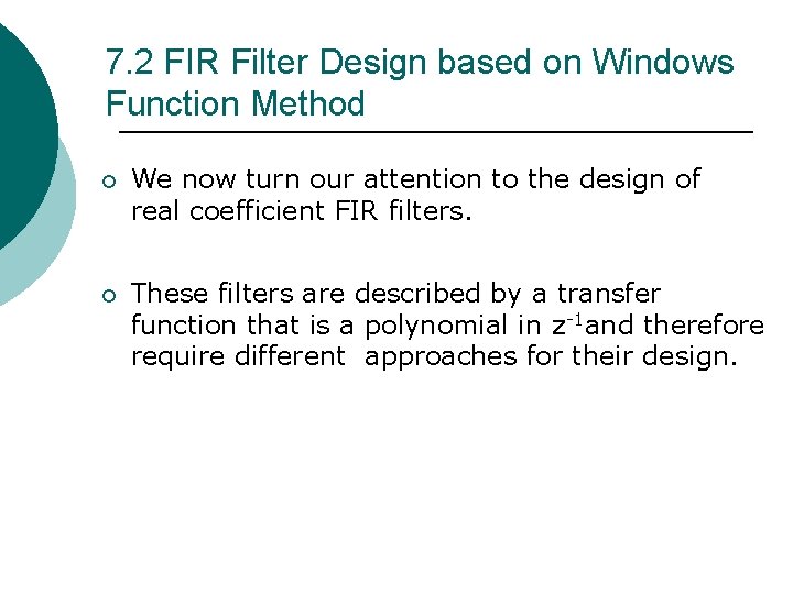
7. 2 FIR Filter Design based on Windows Function Method ¡ We now turn our attention to the design of real coefficient FIR filters. ¡ These filters are described by a transfer function that is a polynomial in z-1 and therefore require different approaches for their design.

7. 2 FIR Filter Design based on Windows Function Method ¡ A direct and straightforward method is based on truncating the Fourier series representation of the prescribed frequency response is discussed in this section.

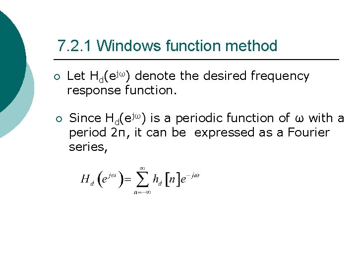
7. 2. 1 Windows function method ¡ Let Hd(ejω) denote the desired frequency response function. ¡ Since Hd(ejω) is a periodic function of ω with a period 2π, it can be expressed as a Fourier series,

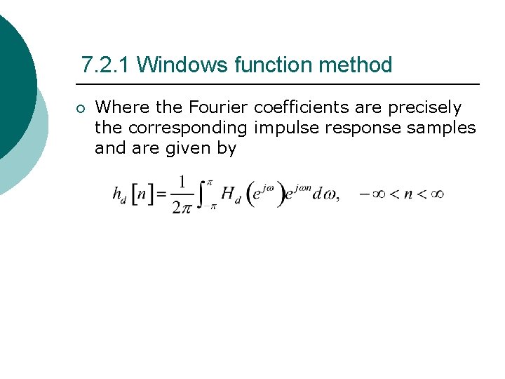
7. 2. 1 Windows function method ¡ Where the Fourier coefficients are precisely the corresponding impulse response samples and are given by

7. 2. 1 Windows function method ¡ Thus, given a frequency response specification Hd(ejω), we can compute hd[n] using the above equation and, hence, determine the transfer function Hd(z). ¡ However, for most practical applications, the desired frequency response is piecewise constant with sharp transitions between bands, in which case, the corresponding impulse response sequence {hd[n]} is of infinite length and noncausal.

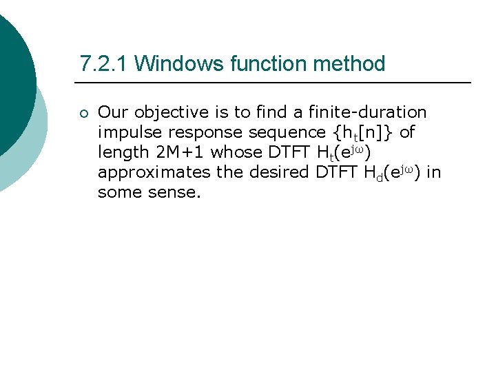
7. 2. 1 Windows function method ¡ Our objective is to find a finite-duration impulse response sequence {ht[n]} of length 2 M+1 whose DTFT Ht(ejω) approximates the desired DTFT Hd(ejω) in some sense.

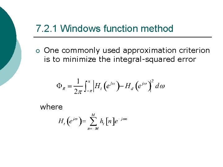
7. 2. 1 Windows function method ¡ One commonly used approximation criterion is to minimize the integral-squared error where

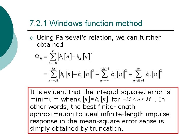
7. 2. 1 Windows function method ¡ Using Parseval’s relation, we can further obtained It is evident that the integral-squared error is minimum when for. In other words, the best finite-length approximation to ideal infinite-length impulse response in the mean-square error sense is simply obtained by truncation.

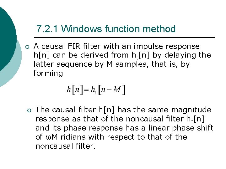
7. 2. 1 Windows function method ¡ ¡ A causal FIR filter with an impulse response h[n] can be derived from ht[n] by delaying the latter sequence by M samples, that is, by forming The causal filter h[n] has the same magnitude response as that of the noncausal filter ht[n] and its phase response has a linear phase shift of ωM ridians with respect to that of the noncausal filter.

7. 2. 2 impulse Response of Ideal Filters ¡ Ideal frequency selective filters are characterized by passband stopband with sharp transitions from passband to stopband. ¡ Four such commonly used filters are the lowpass, highpass, bandpass, and bandstop filters whose ideal frequency response have been discussed.

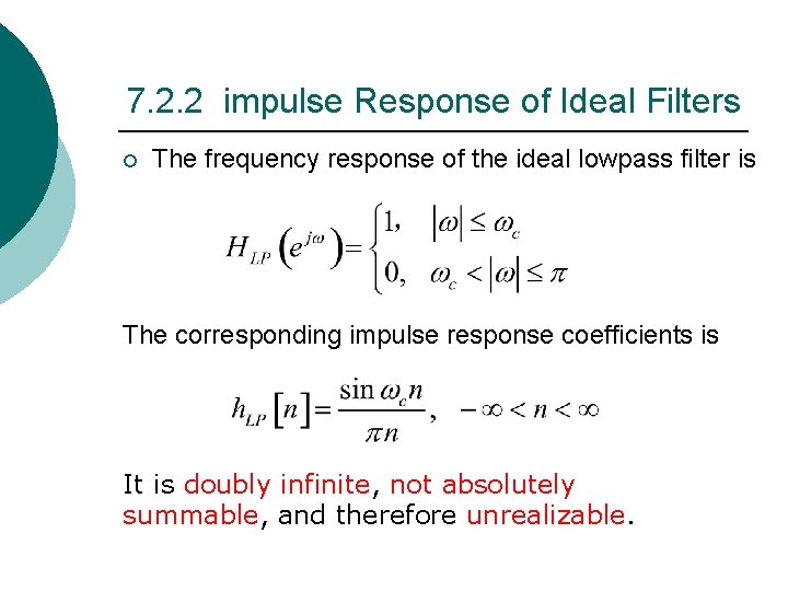
7. 2. 2 impulse Response of Ideal Filters ¡ The frequency response of the ideal lowpass filter is The corresponding impulse response coefficients is It is doubly infinite, not absolutely summable, and therefore unrealizable.

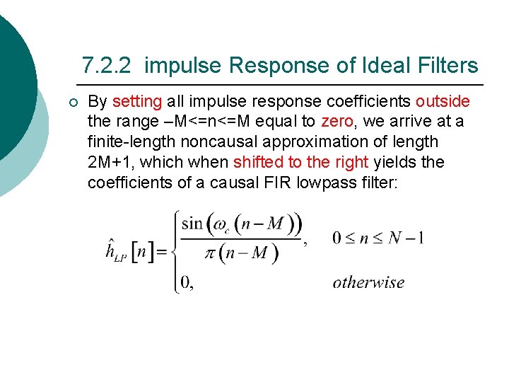
7. 2. 2 impulse Response of Ideal Filters ¡ By setting all impulse response coefficients outside the range –M<=n<=M equal to zero, we arrive at a finite-length noncausal approximation of length 2 M+1, which when shifted to the right yields the coefficients of a causal FIR lowpass filter:

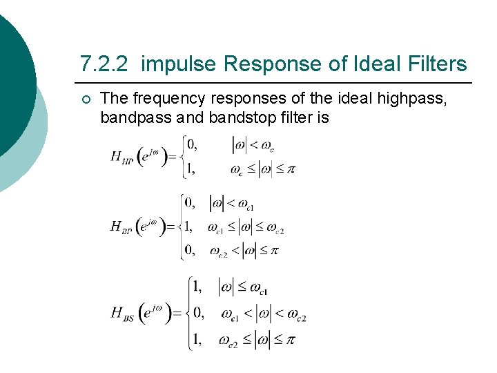
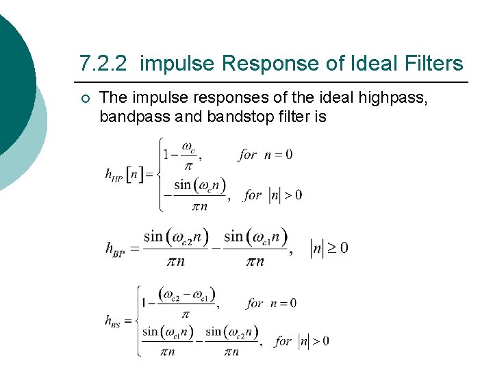
7. 2. 2 impulse Response of Ideal Filters ¡ The frequency responses of the ideal highpass, bandpass and bandstop filter is

7. 2. 2 impulse Response of Ideal Filters ¡ The impulse responses of the ideal highpass, bandpass and bandstop filter is

7. 2. 2 impulse Response of Ideal Filters ¡ They are also characterized by doubly infinite impulse response that are not absolutely summable, making them unrealizable. ¡ They can be made realizable by truncating the impulse response sequence to finite lengths and shifting the truncated coefficients to the right appropriately.

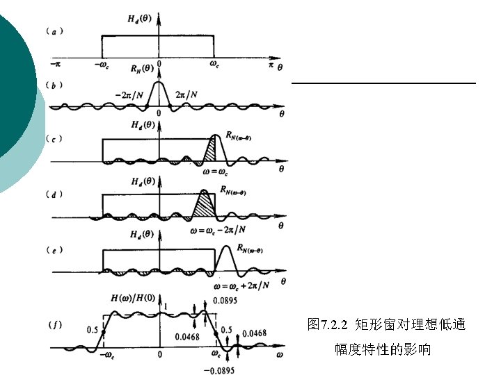
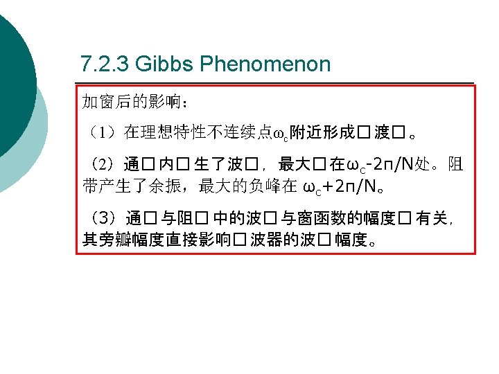
7. 2. 3 Gibbs Phenomenon ¡ The causal FIR filters obtained by simply truncating the impulse response coefficients of the ideal filters given in the previous section exhibit an oscillatory behavior in their respective magnitude responses, which is more commonly referred to as the Gibbs phenomenon.

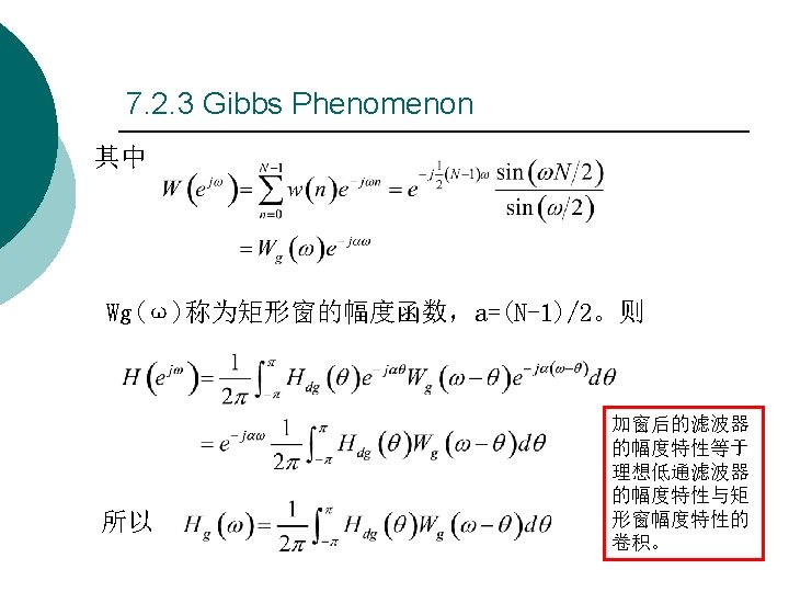
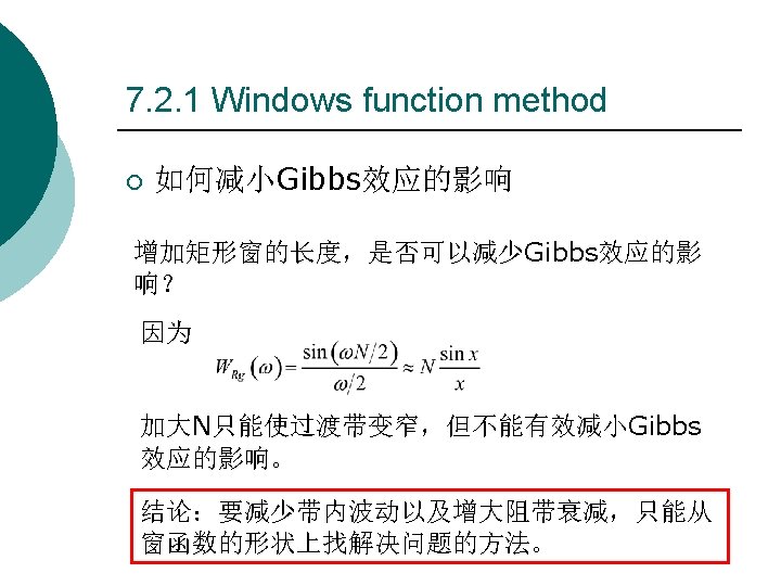
7. 2. 3 Gibbs Phenomenon ¡ The reason behind the Gibbs phenomenon can be explained by considering the truncation operation as multiplication by a finite-length window sequence w[n] and by examining the windowing process in the frequency domain.

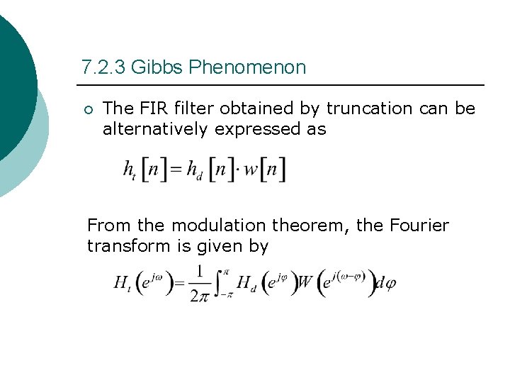
7. 2. 3 Gibbs Phenomenon ¡ The FIR filter obtained by truncation can be alternatively expressed as From the modulation theorem, the Fourier transform is given by

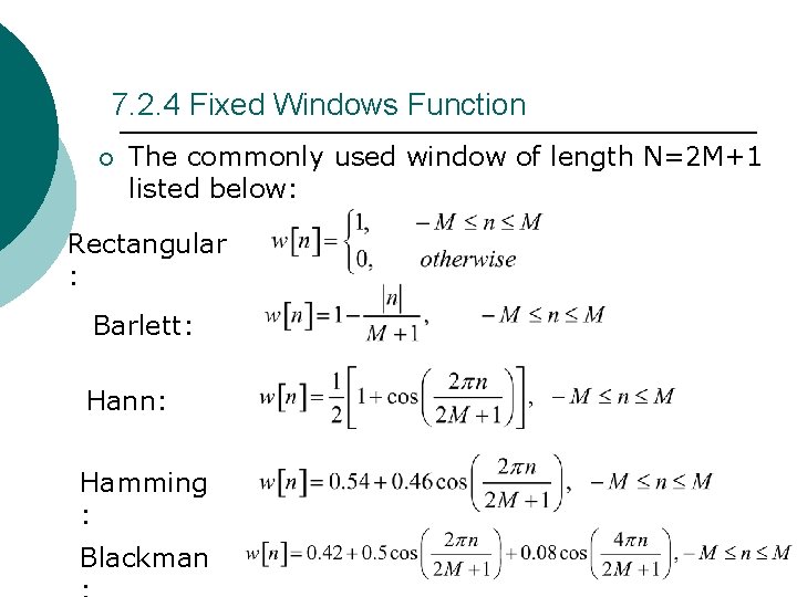
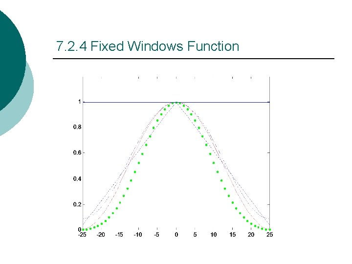
7. 2. 4 Fixed Windows Function ¡ The commonly used window of length N=2 M+1 listed below: Rectangular : Barlett: Hann: Hamming : Blackman

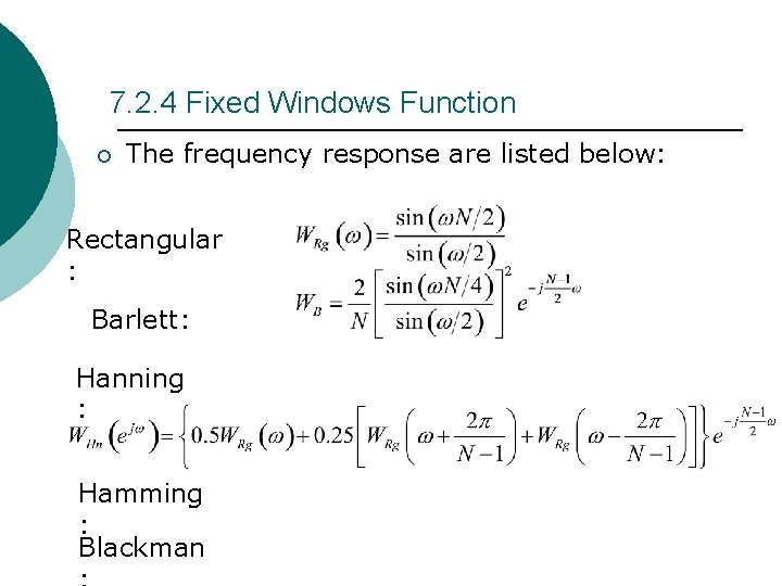
7. 2. 4 Fixed Windows Function ¡ The frequency response are listed below: Rectangular : Barlett: Hanning : Hamming : Blackman

7. 2. 4 Fixed Windows Function

7. 2. 4 Fixed Windows Function

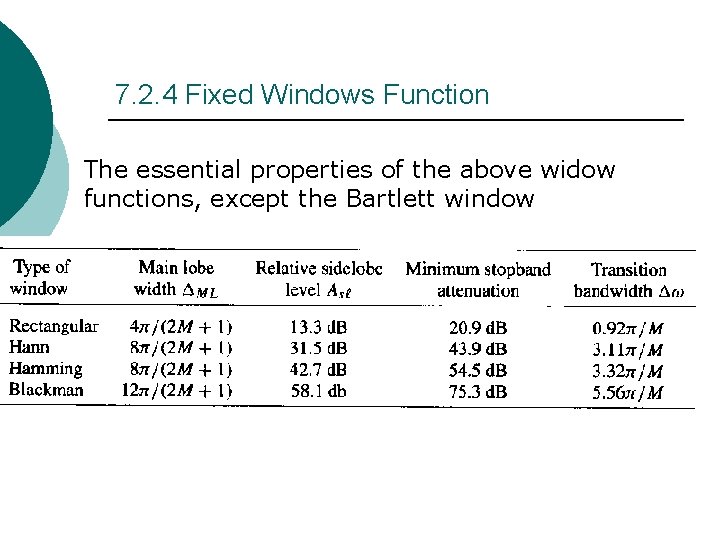
7. 2. 4 Fixed Windows Function The essential properties of the above widow functions, except the Bartlett window

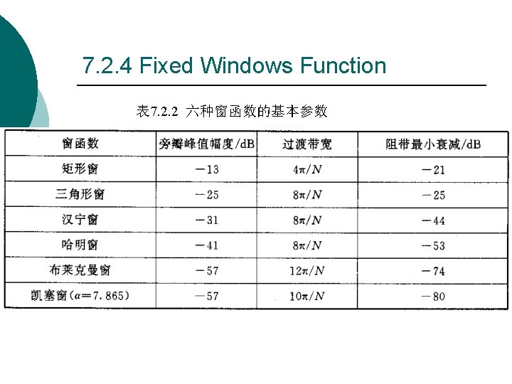
7. 2. 4 Fixed Windows Function 表 7. 2. 2 六种窗函数的基本参数

7. 2. 4 Fixed Windows Function ¡ In the case of the window function of Rectangular, Hann and Hamming, the value of the ripple δ does not depend on the filter length, or the cutoff frequency ωc, and is essentially constant.

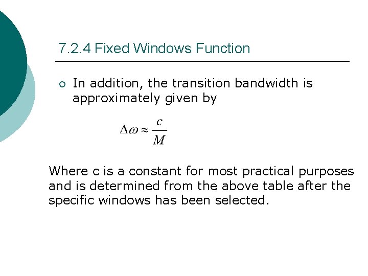
7. 2. 4 Fixed Windows Function ¡ In addition, the transition bandwidth is approximately given by Where c is a constant for most practical purposes and is determined from the above table after the specific windows has been selected.

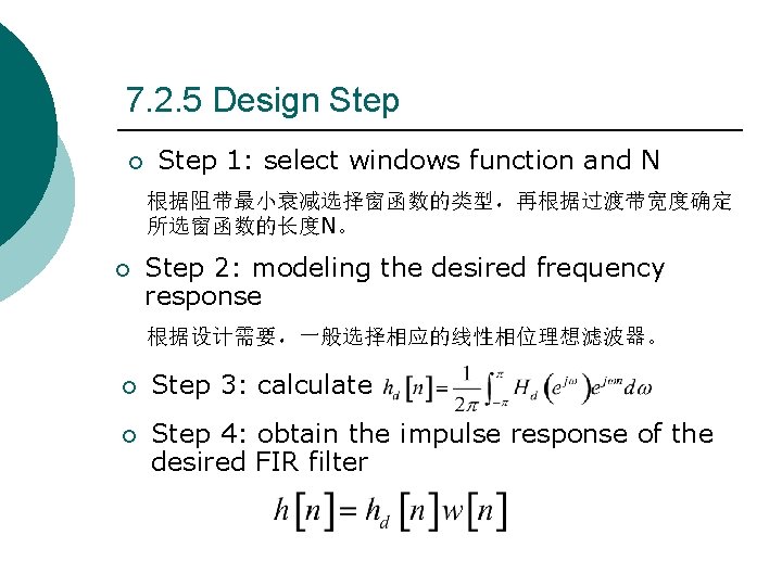
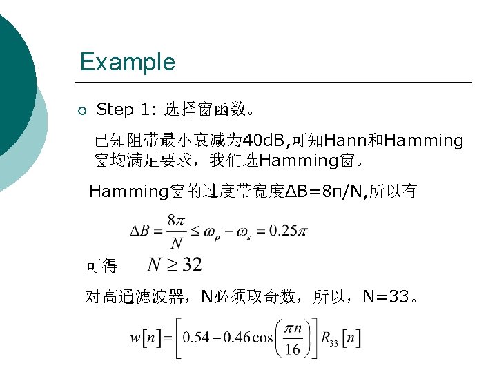
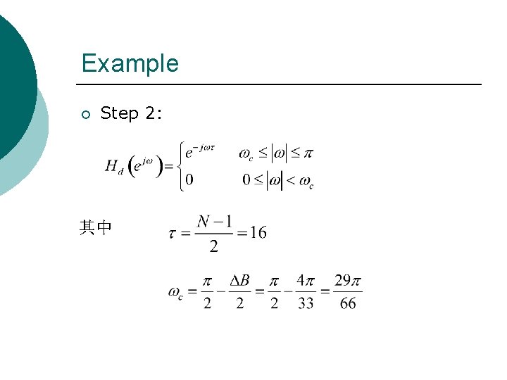
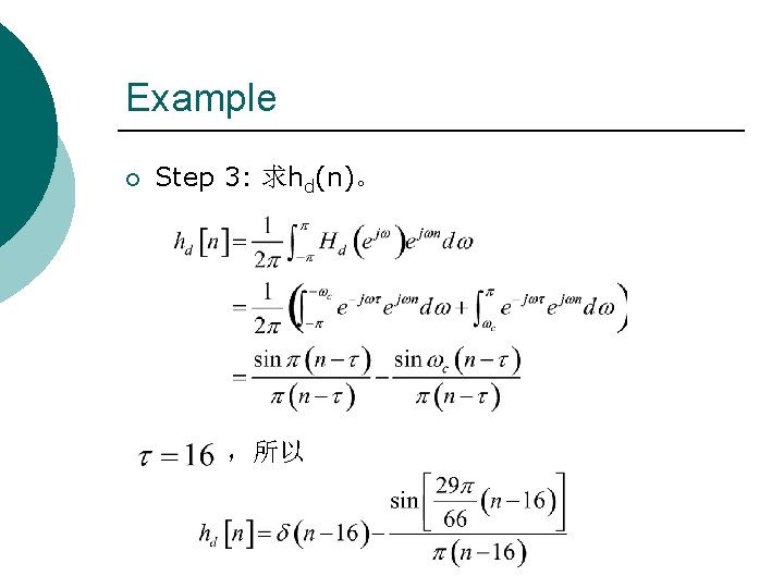
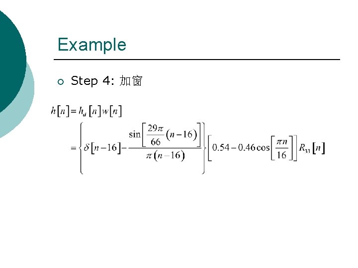
7. 2. 5 Design Step ¡ Step 1: select windows function and N 根据阻带最小衰减选择窗函数的类型，再根据过渡带宽度确定 所选窗函数的长度N。 ¡ Step 2: modeling the desired frequency response 根据设计需要，一般选择相应的线性相位理想滤波器。 ¡ Step 3: calculate ¡ Step 4: obtain the impulse response of the desired FIR filter

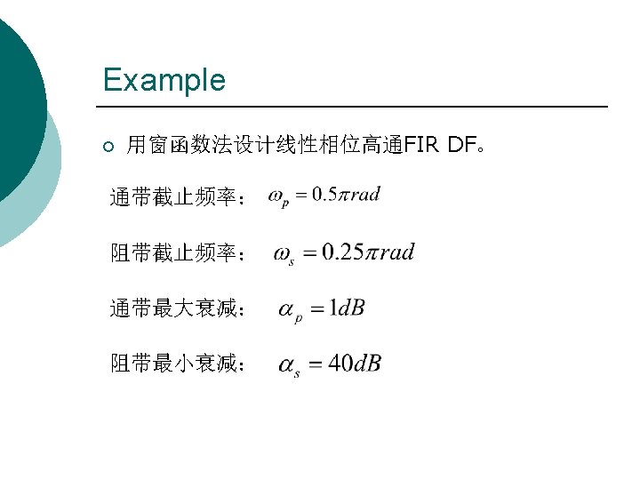
Example ¡ Step 2: 其中

Example ¡ Step 3: 求hd(n)。 ，所以

Example ¡ Step 4: 加窗

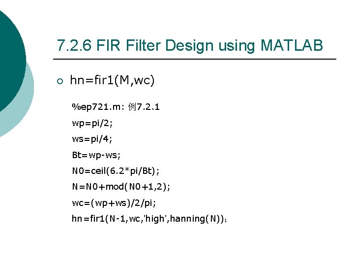
7. 2. 6 FIR Filter Design using MATLAB ¡ hn=fir 1(M, wc) %ep 721. m: 例7. 2. 1 wp=pi/2; ws=pi/4; Bt=wp-ws; N 0=ceil(6. 2*pi/Bt); N=N 0+mod(N 0+1, 2); wc=(wp+ws)/2/pi; hn=fir 1(N-1, wc, ’high’, hanning(N))；

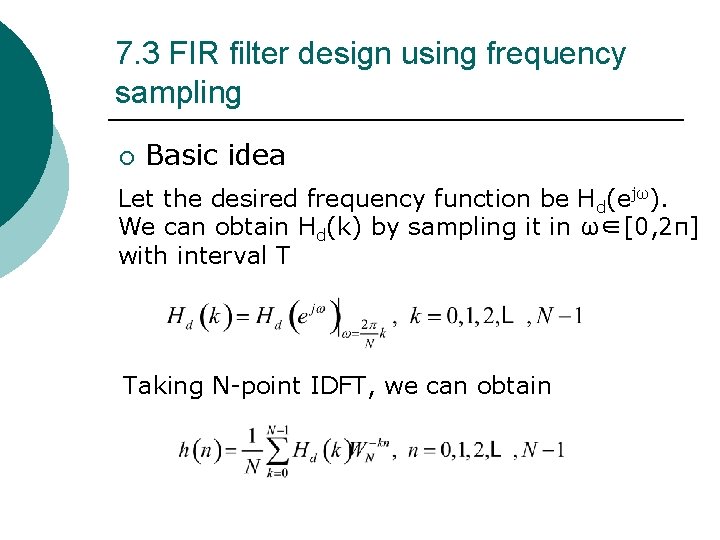
7. 3 FIR filter design using frequency sampling ¡ Basic idea Let the desired frequency function be Hd(ejω). We can obtain Hd(k) by sampling it in ω∈[0, 2π] with interval T Taking N-point IDFT, we can obtain

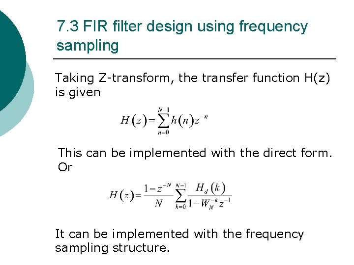
7. 3 FIR filter design using frequency sampling Taking Z-transform, the transfer function H(z) is given This can be implemented with the direct form. Or It can be implemented with the frequency sampling structure.

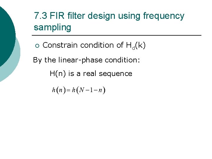
7. 3 FIR filter design using frequency sampling ¡ Constrain condition of Hd(k) By the linear-phase condition: H(n) is a real sequence

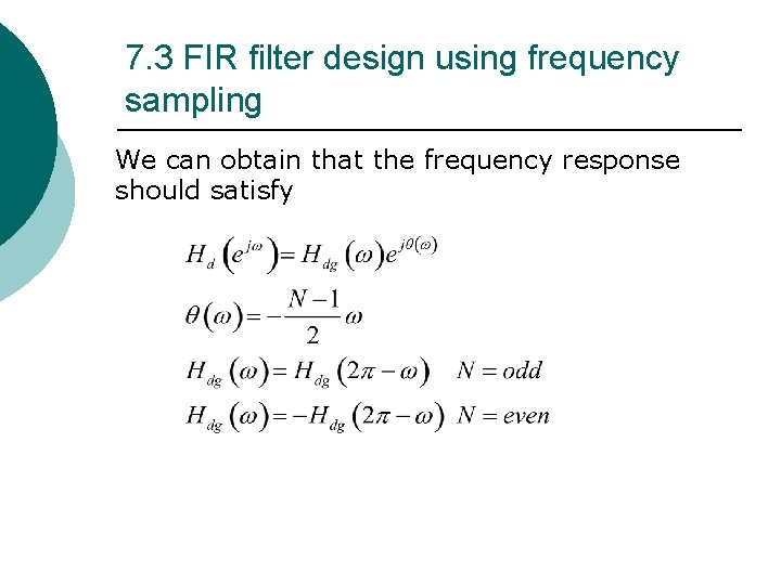
7. 3 FIR filter design using frequency sampling We can obtain that the frequency response should satisfy

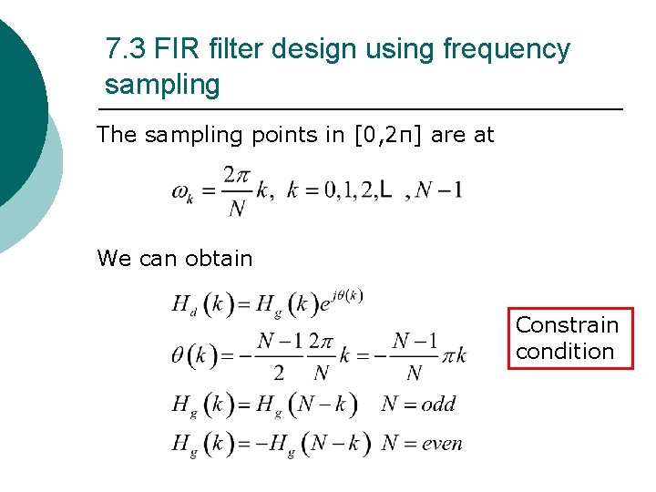
7. 3 FIR filter design using frequency sampling The sampling points in [0, 2π] are at We can obtain Constrain condition

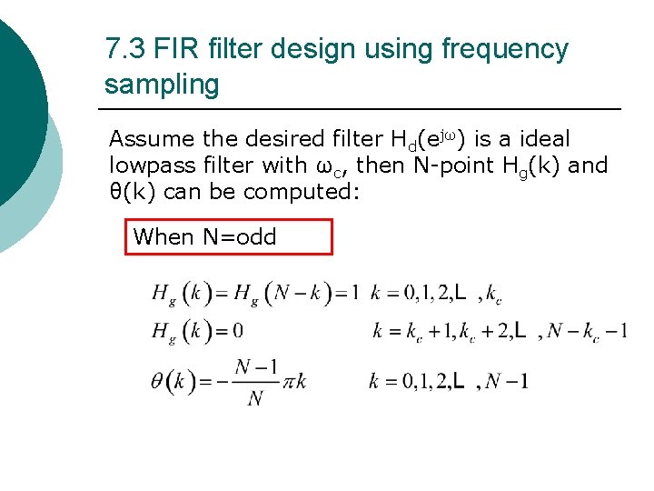
7. 3 FIR filter design using frequency sampling Assume the desired filter Hd(ejω) is a ideal lowpass filter with ωc, then N-point Hg(k) and θ(k) can be computed: When N=odd

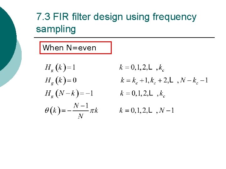
7. 3 FIR filter design using frequency sampling When N=even

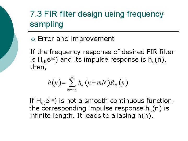
7. 3 FIR filter design using frequency sampling ¡ Error and improvement If the frequency response of desired FIR filter is Hd(ejω) and its impulse response is hd(n), then, If Hd(ejω) is not a smooth continuous function, the corresponding impulse response hd(n) is infinite length. It leads to aliasing h(n).

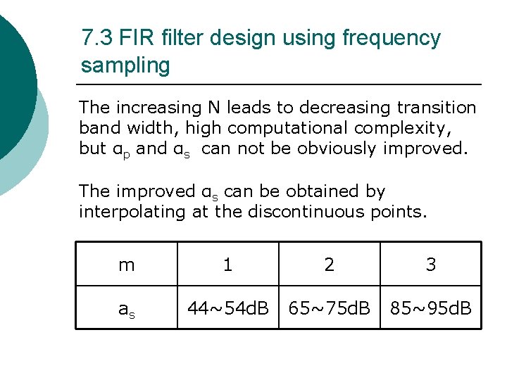
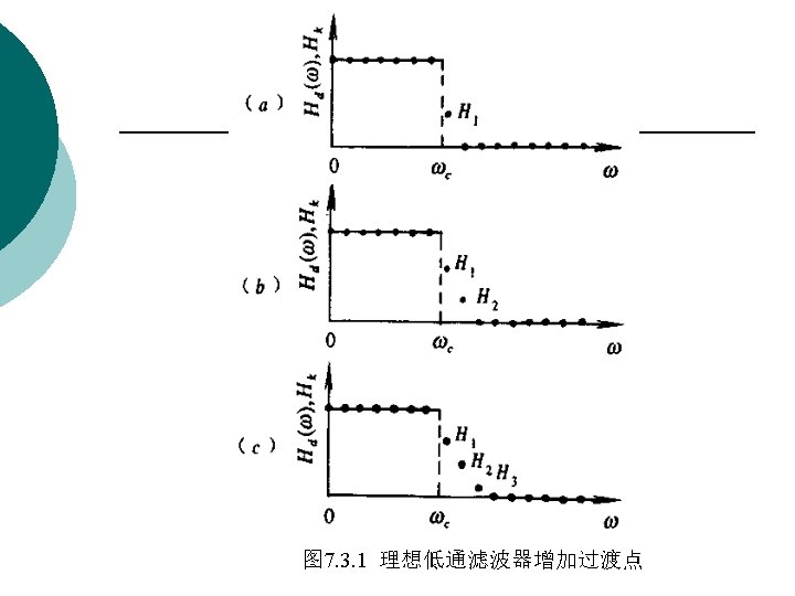
7. 3 FIR filter design using frequency sampling The increasing N leads to decreasing transition band width, high computational complexity, but αp and αs can not be obviously improved. The improved αs can be obtained by interpolating at the discontinuous points. m 1 2 3 as 44~54 d. B 65~75 d. B 85~95 d. B

7. 3 FIR filter design using frequency sampling ¡ Examples See P 220

7. 4 Computer-Aided Design of Equiripple Linear-Phase FIR Filters ¡ In this section, we consider the application of computer-aided optimization technique for the design of FIR filters.

7. 4 Computer-Aided Design of Equiripple Linear-Phase FIR Filters ¡ The basic idea behind the computer-based technique is to minimize iteratively an error measure that is function of the difference between the desired frequency response D(ejω) and the frequency response H(ejω) of the filter being designed.

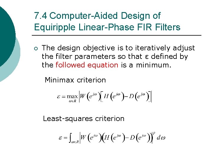
7. 4 Computer-Aided Design of Equiripple Linear-Phase FIR Filters ¡ The design objective is to iteratively adjust the filter parameters so that ε defined by the followed equation is a minimum. Minimax criterion Least-squares criterion

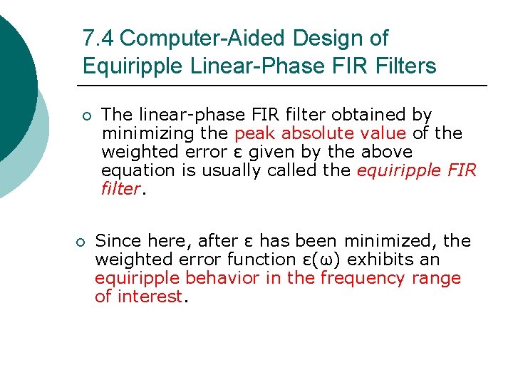
7. 4 Computer-Aided Design of Equiripple Linear-Phase FIR Filters ¡ ¡ The linear-phase FIR filter obtained by minimizing the peak absolute value of the weighted error ε given by the above equation is usually called the equiripple FIR filter. Since here, after ε has been minimized, the weighted error function ε(ω) exhibits an equiripple behavior in the frequency range of interest.

The Parks-Mc. Clellan Algorithm ¡ A weighted-Chebyshev approximation method has been advanced by Parks and Mc. Clellan for designing equiripple liearphase FIR filters.

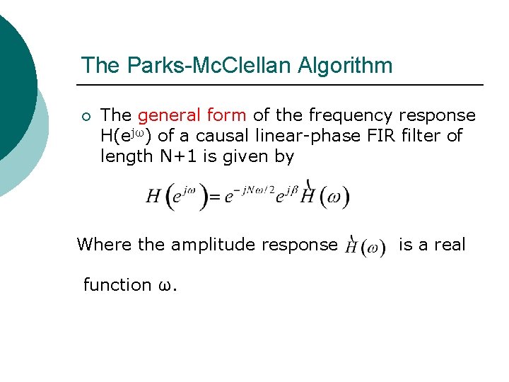
The Parks-Mc. Clellan Algorithm ¡ The general form of the frequency response H(ejω) of a causal linear-phase FIR filter of length N+1 is given by Where the amplitude response function ω. is a real

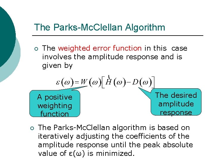
The Parks-Mc. Clellan Algorithm ¡ The weighted error function in this case involves the amplitude response and is given by A positive weighting function ¡ The desired amplitude response The Parks-Mc. Clellan algorithm is based on iteratively adjusting the coefficients of the amplitude response until the peak absolute value of ε(ω) is minimized.

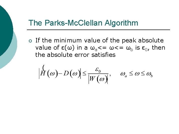
The Parks-Mc. Clellan Algorithm ¡ If the minimum value of the peak absolute value of ε(ω) in a ωa<= ωb is ε 0, then the absolute error satisfies

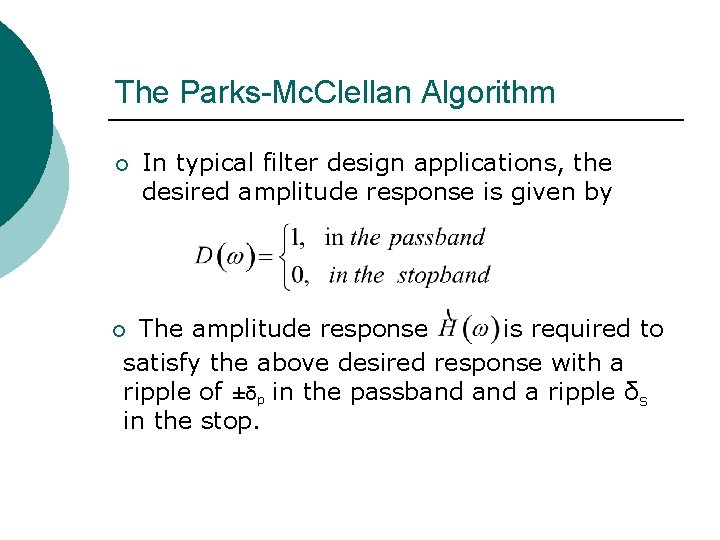
The Parks-Mc. Clellan Algorithm ¡ In typical filter design applications, the desired amplitude response is given by The amplitude response is required to satisfy the above desired response with a ripple of ±δp in the passband a ripple δs in the stop. ¡

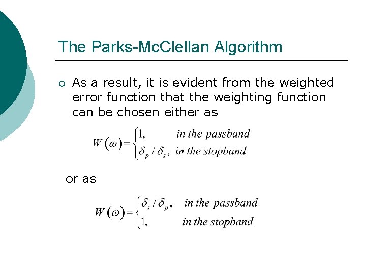
The Parks-Mc. Clellan Algorithm ¡ As a result, it is evident from the weighted error function that the weighting function can be chosen either as or as

The Parks-Mc. Clellan Algorithm ¡ ¡ ¡ By a clever manipulation, the expression for the amplitude response for each of the four types of linear-phase FIR filters can be expressed in the same form. The same algorithm can be adapted to design any one of the four types of filters. To develop this general form for the amplitude response expression, we consider each of the four types of filters separately.

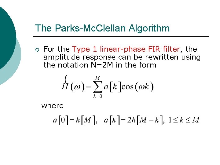
The Parks-Mc. Clellan Algorithm ¡ For the Type 1 linear-phase FIR filter, the amplitude response can be rewritten using the notation N=2 M in the form where

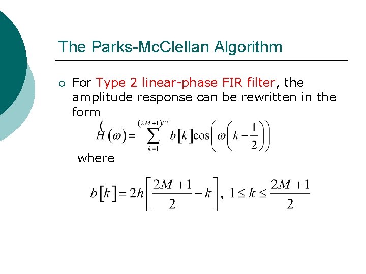
The Parks-Mc. Clellan Algorithm ¡ For Type 2 linear-phase FIR filter, the amplitude response can be rewritten in the form where

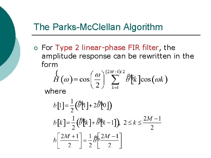
The Parks-Mc. Clellan Algorithm ¡ For Type 2 linear-phase FIR filter, the amplitude response can be rewritten in the form where

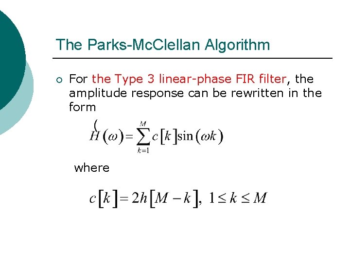
The Parks-Mc. Clellan Algorithm ¡ For the Type 3 linear-phase FIR filter, the amplitude response can be rewritten in the form where

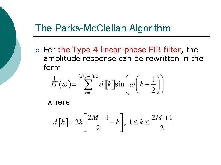
The Parks-Mc. Clellan Algorithm ¡ For the Type 4 linear-phase FIR filter, the amplitude response can be rewritten in the form where

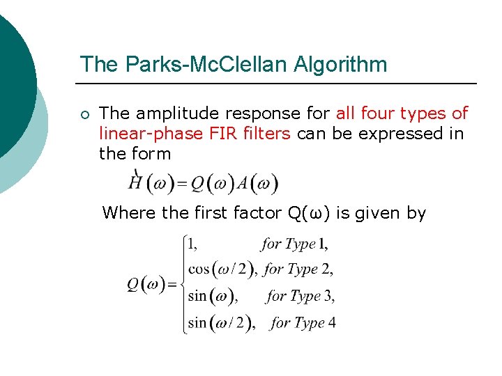
The Parks-Mc. Clellan Algorithm ¡ The amplitude response for all four types of linear-phase FIR filters can be expressed in the form Where the first factor Q(ω) is given by

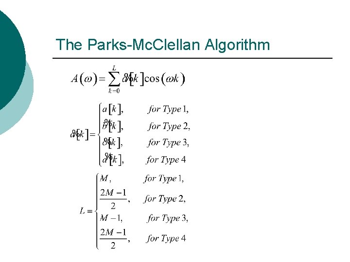
The Parks-Mc. Clellan Algorithm

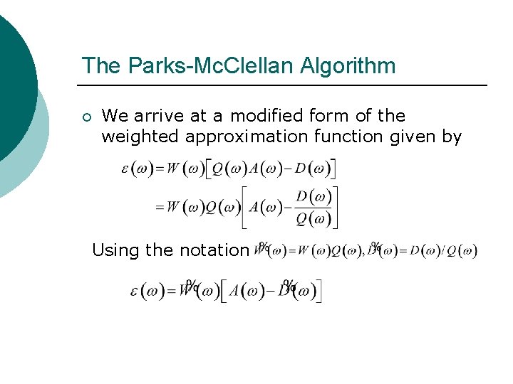
The Parks-Mc. Clellan Algorithm ¡ We arrive at a modified form of the weighted approximation function given by Using the notation

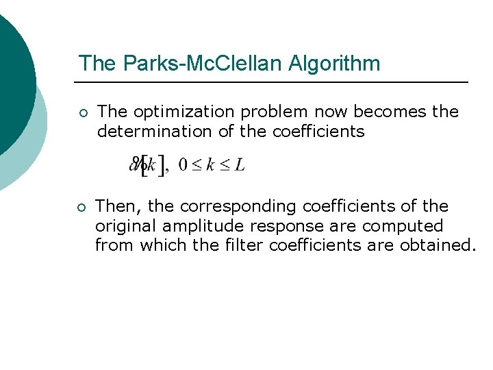
The Parks-Mc. Clellan Algorithm ¡ The optimization problem now becomes the determination of the coefficients ¡ Then, the corresponding coefficients of the original amplitude response are computed from which the filter coefficients are obtained.

Alteration Theorem ¡ The amplitude function A(ω) is the best unique approximation of the desired amplitude response obtained by minimizing the peak absolute valueεof ε(ω) if and only if there exist at least L+2 extremal angular frequencies.

The Parks-Mc. Clellan Algorithm ¡ The Remez exchange algrithm, a highly efficient iterative procedure, is used to determine the locations of the extremal frequencies and consists of the following steps at each iteration stage:

The Parks-Mc. Clellan Algorithm ¡ Step 1: A set of initial value for the extremal frequencies are either chosen or are available from the completion of the previous iteration.

The Parks-Mc. Clellan Algorithm ¡ Step 2: The value ε is then computed by solving the following equation

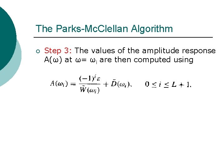
The Parks-Mc. Clellan Algorithm ¡ Step 3: The values of the amplitude response A(ω) at ω= ωi are then computed using

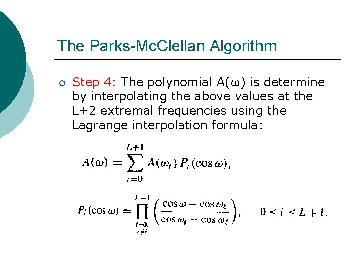
The Parks-Mc. Clellan Algorithm ¡ Step 4: The polynomial A(ω) is determine by interpolating the above values at the L+2 extremal frequencies using the Lagrange interpolation formula:

The Parks-Mc. Clellan Algorithm ¡ Step 5: The new weighted error function ε(ω) is computed at a dense set S(S>=L) of frequencies. In practice, S=16 L is adequate. Determine the L+2 new extremal frequencies from the values of ε(ω) evaluated at the dense set of frequencies.

The Parks-Mc. Clellan Algorithm ¡ Step 6: If the peak values ε are equal in magnitude, the algorithm has converged. Otherwise, go bask to Step 2.

10. 5 FIR Digital Filter Design Using MATLAB ¡ The signal Processing Tool. Box of MATLAB includes a variety of M-files for the design of FIR digital filters.

10. 5. 1 FIR Digital Filter Order Estimation Using MATLAB ¡ As in the case of FIR digital filter design, the FIR digital filter design process also consists of two steps. ¡ In the first step, the filter order is estimated from the given specification ¡ In the second step, the coefficients of the transfer function are determined using the estimated order and filter specifications. .

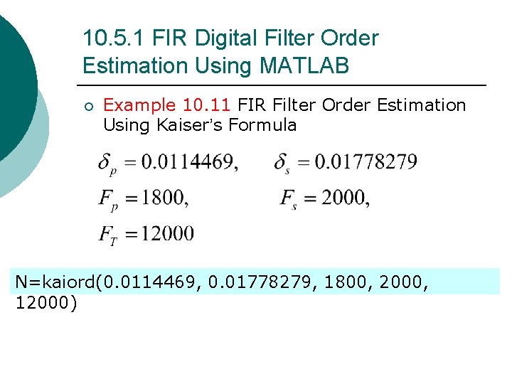
10. 5. 1 FIR Digital Filter Order Estimation Using MATLAB ¡ Example 10. 11 FIR Filter Order Estimation Using Kaiser’s Formula N=kaiord(0. 0114469, 0. 01778279, 1800, 2000, 12000)

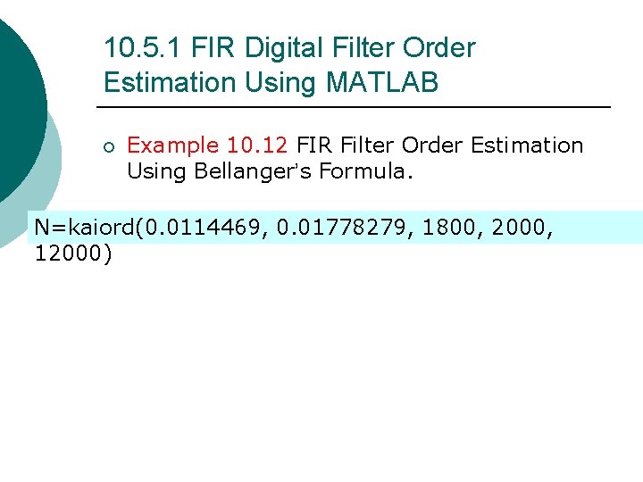
10. 5. 1 FIR Digital Filter Order Estimation Using MATLAB ¡ Example 10. 12 FIR Filter Order Estimation Using Bellanger’s Formula. N=kaiord(0. 0114469, 0. 01778279, 1800, 2000, 12000)

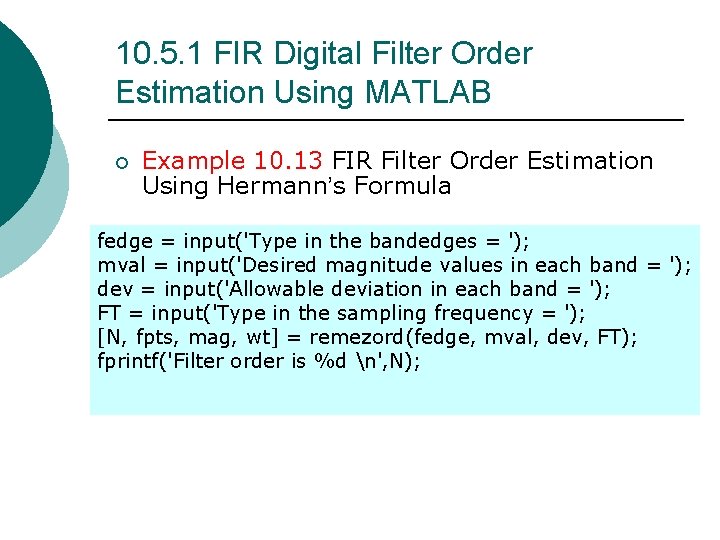
10. 5. 1 FIR Digital Filter Order Estimation Using MATLAB ¡ Example 10. 13 FIR Filter Order Estimation Using Hermann’s Formula fedge = input('Type in the bandedges = '); mval = input('Desired magnitude values in each band = '); dev = input('Allowable deviation in each band = '); FT = input('Type in the sampling frequency = '); [N, fpts, mag, wt] = remezord(fedge, mval, dev, FT); fprintf('Filter order is %d n', N);

10. 5. 2 Equiripple Linear-Phase FIR Filter Design Using MATLAB ¡ For designing an equiripple linear-phase FIR filter employing the Parks-Mc. Clellan algorithm, we can use the MATLAB M-files remez.

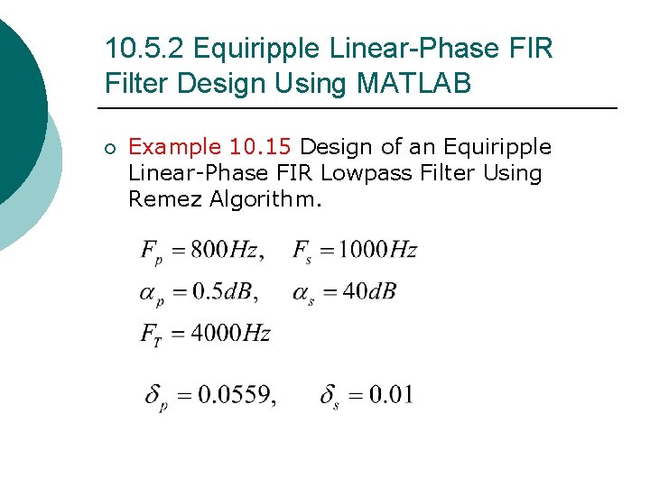
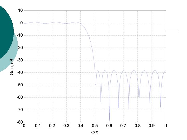
10. 5. 2 Equiripple Linear-Phase FIR Filter Design Using MATLAB ¡ Example 10. 15 Design of an Equiripple Linear-Phase FIR Lowpass Filter Using Remez Algorithm.

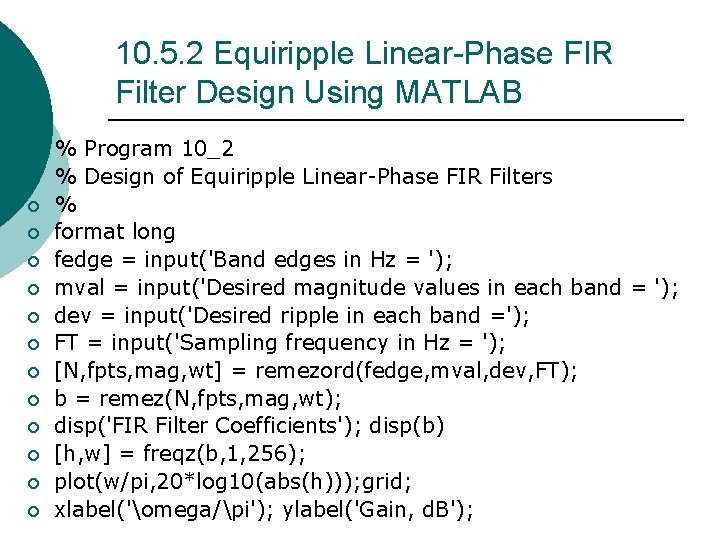
10. 5. 2 Equiripple Linear-Phase FIR Filter Design Using MATLAB ¡ ¡ ¡ ¡ % Program 10_2 % Design of Equiripple Linear-Phase FIR Filters % format long fedge = input('Band edges in Hz = '); mval = input('Desired magnitude values in each band = '); dev = input('Desired ripple in each band ='); FT = input('Sampling frequency in Hz = '); [N, fpts, mag, wt] = remezord(fedge, mval, dev, FT); b = remez(N, fpts, mag, wt); disp('FIR Filter Coefficients'); disp(b) [h, w] = freqz(b, 1, 256); plot(w/pi, 20*log 10(abs(h))); grid; xlabel('omega/pi'); ylabel('Gain, d. B');

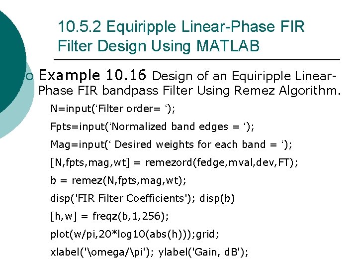
10. 5. 2 Equiripple Linear-Phase FIR Filter Design Using MATLAB ¡ Example 10. 16 Design of an Equiripple Linear- Phase FIR bandpass Filter Using Remez Algorithm. N=input(‘Filter order= ‘); Fpts=input(‘Normalized band edges = ‘); Mag=input(‘ Desired weights for each band = ‘); [N, fpts, mag, wt] = remezord(fedge, mval, dev, FT); b = remez(N, fpts, mag, wt); disp('FIR Filter Coefficients'); disp(b) [h, w] = freqz(b, 1, 256); plot(w/pi, 20*log 10(abs(h))); grid; xlabel('omega/pi'); ylabel('Gain, d. B');

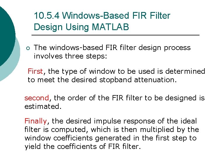
10. 5. 4 Windows-Based FIR Filter Design Using MATLAB ¡ The windows-based FIR filter design process involves three steps: First, the type of window to be used is determined to meet the desired stopband attenuation. second, the order of the FIR filter to be designed is estimated. Finally, the desired impulse response of the ideal filter is computed, which is then multiplied by the window coefficients generated in the first step to yield the coefficients of FIR filter.

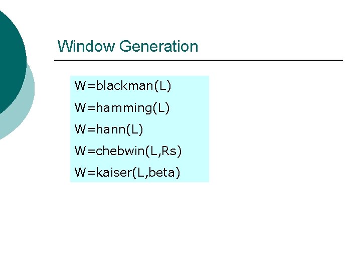
Window Generation W=blackman(L) W=hamming(L) W=hann(L) W=chebwin(L, Rs) W=kaiser(L, beta)

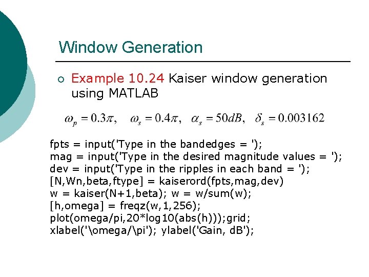
Window Generation ¡ Example 10. 24 Kaiser window generation using MATLAB fpts = input('Type in the bandedges = '); mag = input('Type in the desired magnitude values = '); dev = input('Type in the ripples in each band = '); [N, Wn, beta, ftype] = kaiserord(fpts, mag, dev) w = kaiser(N+1, beta); w = w/sum(w); [h, omega] = freqz(w, 1, 256); plot(omega/pi, 20*log 10(abs(h))); grid; xlabel('omega/pi'); ylabel('Gain, d. B');

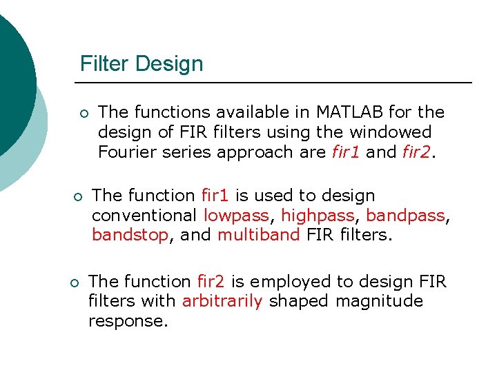
Filter Design ¡ ¡ ¡ The functions available in MATLAB for the design of FIR filters using the windowed Fourier series approach are fir 1 and fir 2. The function fir 1 is used to design conventional lowpass, highpass, bandstop, and multiband FIR filters. The function fir 2 is employed to design FIR filters with arbitrarily shaped magnitude response.

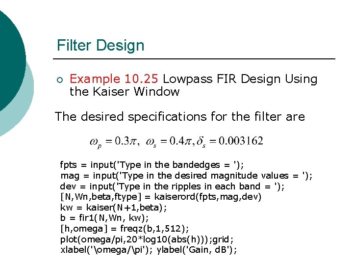
Filter Design ¡ Example 10. 25 Lowpass FIR Design Using the Kaiser Window The desired specifications for the filter are fpts = input('Type in the bandedges = '); mag = input('Type in the desired magnitude values = '); dev = input('Type in the ripples in each band = '); [N, Wn, beta, ftype] = kaiserord(fpts, mag, dev) kw = kaiser(N+1, beta); b = fir 1(N, Wn, kw); [h, omega] = freqz(b, 1, 512); plot(omega/pi, 20*log 10(abs(h))); grid; xlabel('omega/pi'); ylabel('Gain, d. B');

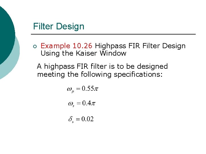
Filter Design ¡ Example 10. 26 Highpass FIR Filter Design Using the Kaiser Window A highpass FIR filter is to be designed meeting the following specifications:

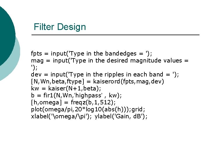
Filter Design fpts = input('Type in the bandedges = '); mag = input('Type in the desired magnitude values = '); dev = input('Type in the ripples in each band = '); [N, Wn, beta, ftype] = kaiserord(fpts, mag, dev) kw = kaiser(N+1, beta); b = fir 1(N, Wn, ’highpass’ , kw); [h, omega] = freqz(b, 1, 512); plot(omega/pi, 20*log 10(abs(h))); grid; xlabel('omega/pi'); ylabel('Gain, d. B');

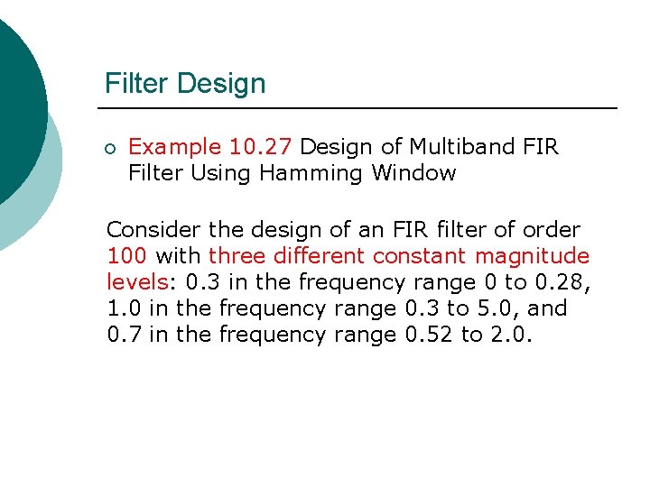
Filter Design ¡ Example 10. 27 Design of Multiband FIR Filter Using Hamming Window Consider the design of an FIR filter of order 100 with three different constant magnitude levels: 0. 3 in the frequency range 0 to 0. 28, 1. 0 in the frequency range 0. 3 to 5. 0, and 0. 7 in the frequency range 0. 52 to 2. 0.

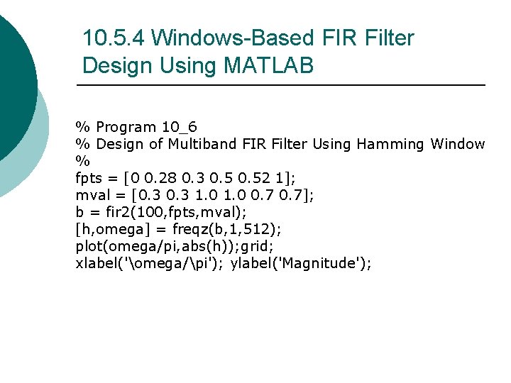
10. 5. 4 Windows-Based FIR Filter Design Using MATLAB % Program 10_6 % Design of Multiband FIR Filter Using Hamming Window % fpts = [0 0. 28 0. 3 0. 52 1]; mval = [0. 3 1. 0 0. 7]; b = fir 2(100, fpts, mval); [h, omega] = freqz(b, 1, 512); plot(omega/pi, abs(h)); grid; xlabel('omega/pi'); ylabel('Magnitude');