Chapter 6 IIR Digital Filter Design Introduce l

Chapter 6 IIR Digital Filter Design

Introduce l Digital Filter -- One of the most widely used complex signal processing operations is filtering, whose main objective is to alter the spectrum according to some given specifications. The system implementing this operation is called a filter. The discrete-time system for the treatment of discrete-time signal is called a digital filter. *

Introduce l Classification of Digital Filter According to the characterization of the eliminated frequency component, the digital filters are usually classified as: u Classical filters The useful frequency components in input signal are different from the eliminated frequency components. u Modern filters The signal is aliased into interferer frequency component. *

Introduce l Classification of Digital Filter u * According to magnitude characteristics of the transfer function, the Classical filters include: p Lowpass filters p Highpass filters p Bandstop filters.

Introduce According to the length of their impulse response sequences, the digital filters are usually classified as: u Infinite impulse response (IIR) filters u Finite impulse response (FIR) filters *

Introduce ¡ An important step in the development of a digital filter is the determination of a realizable transfer function H(z) approximating the given frequency response specifications. The process of deriving the transfer function H(z) is called digital filter design. *

Introduce * ¡ In Chapter 5, we outlined a variety of basic structures for the realization of IIR and FIR transfer functions. ¡ In this chapter, we consider the IIR digital filter design problem. The design of FIR digital filters is discussed in Chapter 7.

Content * l Digital Filter Specifications l Design of analog filters l Impulse Invariance Method of Lowpass IIR Digital Filters Design l Bilinear Transformation Method of Lowpass IIR Digital Filter Design l Design of Highpass, Bandpass and Bandstop Digital Filters

6. 1 Concepts on Digital Filter u There are two major issues that need to be answered before one can develop the digital transfer function G(z). p The first issue is the development of a reasonable filter frequency response specification from the requirements of overall system in which the digital filter is to be designed. p The second issue is to determine whether an FIR or IIR digital filter is to be designed. *

6. 1 Concepts on Digital Filter l Digital Filter Specification ¡ ¡ * As in the case of the design of analog filters, either the magnitude and/or the phase response is specified for the design of a digital filter for most application. In most practical applications, the problem of interest is the development of a realizable approximation to a given magnitude response specification. The phase response of the filter can be corrected by cascading it with an allpass filter.

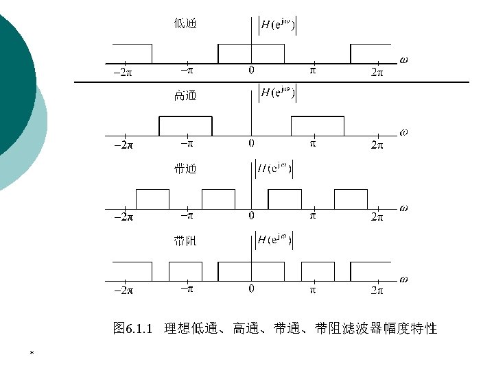
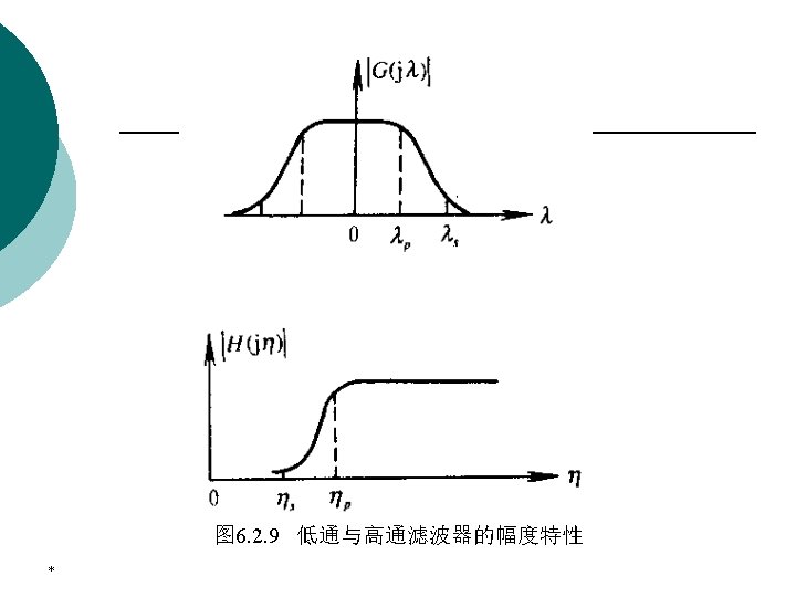
6. 1 Concepts on Digital Filter ¡ * We restrict our attention in this chapter to the magnitude approximation problem only. We pointed out that there are four basic types of filters, whose magnitude responses are shown:

6. 1 Concepts on Digital Filter * ¡ Since the impulse response corresponding to each of these is noncausal and of infinite length, these ideal filters are not realizable. ¡ One way of developing a realizable approximation to these filters would be to truncate the impulse response for a lowpass filter.

6. 1 Concepts on Digital Filter ¡ ¡ ¡ * The magnitude response specifications of a digital filter in passband in the stopband are given with some acceptable tolerances. A transition band is specified between the passband the stopband to permit the magnitude to drop off smoothly. For example, the magnitude of a losspass filter may be given as shown in Figure 9. 1

Peak ripple value Passband edge frequency * Transition band Stopband edge frequency

6. 1 Concepts on Digital Filter Passband defined by Error bound Magnitude Stopband defined by Error bound Magnitude Transition band *

6. 1 Concepts on Digital Filter ¡ Note: The frequency response of a digital filter is a periodic function of ω, and the magnitude response of a real-coefficient digital filter is an even function of ω. As a result, the digital filter specifications are given only for the range *

6. 1 Concepts on Digital Filter ¡ Digital filter specifications are often given in terms of loss function, in d. B. Thus Peak passband ripple Minimum stopband attenuation *

6. 1 Concepts on Digital Filter ¡ The magnitude response specifications for a digital lowpass filter may alternatively be given I a normalized form: Ø Ø Ø * The maximum value of the magnitude in passband is assumed to be unity. The maximum passband deviation, denoted as is given by the minimum value of the magnitude in the passband. The maximum stopband magnitude is denoted by 1/A.

6. 1 Concepts on Digital Filter * Maximum passband attenuation

6. 1 Concepts on Digital Filter ¡ Maximum passband attenuation For * as is typically the case, it can be shown

6. 1 Concepts on Digital Filter ¡ * The passband stopband edge frequencies, in most applications, are specified in Hz, along with the sampling rate of the digital. Then, the normalized angular edge frequencies in radians are given by

6. 1 Concepts on Digital Filter l Selection of the Filter Type * ¡ The second issue of interest is the selection of the digital filter type, that is, whether an IIR or an FIR digital filter is to be employed. ¡ The objective of digital filter design is to develop a causal transfer function H(z) meeting the frequency response specifications.

6. 1 Concepts on Digital Filter ¡ For IIR digital filter design, the transfer function is a rational function of z-1 : Moreover, H(z) must be a stable transfer function, and for reduced computational complexity, it must be of lowest order N. *

6. 1 Concepts on Digital Filter ¡ For FIR filter design, the transfer function is polynomial in z-1 : For reduced computational complexity, the degree N of H(z) must be as small as possible. In addition, if a linear phase is desired, then the FIR filter coefficients must satisfy the constraint: *

6. 1 Concepts on Digital Filter ¡ Advantages in using an FIR filter ØIt can be designed with exact linear phase. ØThe filter structure is always stable with quantized filter coefficients. *

6. 1 Concepts on Digital Filter ¡ Disadvantages in using an FIR filter ØIn the cases, the order NFIR of an FIR filter is considerably higher than the order NIIR of an equivalent IIR filter meeting the same magnitude specification. It has been shown that for most practical filter specifications, the ratio NFIR/NIIR is typically of the order of tens or more and, as a result, the IIR filter usually is computationally more efficient. *

6. 1 Concepts on Digital Filter ¡ ¡ * If the group delay of the IIR filter is equalized by cascading it with an allpass equalizer, then the savings in computation may longer be that significant. In many applications, the linearity of the phase response of the digital filter is not an issue, making the IIR filter preferable because of the lower computational requirements.

6. 1 Concepts on Digital Filter l Introduce of filter design ¡ * The approach to IIR filter design based on the conversion of a prototype analog transfer function to a digital transfer function is widely used. Then, the most common practice of IIR filter design is

6. 1 Concepts on Digital Filter p To convert the digital filter specifications into analog lowpass prototype filter specifications. p To determine the analog lowpass filter transfer function meeting these specifications p To transform it into the desired digital filter transfer function. *

6. 1 Concepts on Digital Filter ¡ Why is this approach used? p Analog approximation techniques are highly advanced. p They usually yield closed-form solutions. p Extensive tables are available for analog filter design. p Many applications require the digital simulation of analog filter. *

6. 1 Concepts on Digital Filter We denote an analog transfer function as The digital transfer function derived from Ha(s) is denoted by *

6. 1 Concepts on Digital Filter ¡ * The basic idea behind the conversion of an analog prototype transfer function Ha(s) into a digital IIR transfer function G(z) is to apply a mapping from the s-domain to the z-domain so that the essential properties of the analog frequency response are preserved.

6. 1 Concepts on Digital Filter ¡ The mapping function should be such that p the imaginary axis in the s-plane be mapping onto the unit circle of the z-plane. p a stable analog transfer function be transformed into a stable digital transfer function. The widely used transformation is the Bilinear Transformation and Impulse Invariance Method. *

6. 2 Analog Filter Design

1. Introduce ¡ * There a number of established approximation techniques for the design of analog lowpass filters. Here we describe four widely used design techniques without their detailed derivations. Further details of these methods can be found in texts on analog filter design.

1. Introduce Filter specifications ¡ Butterworth approximation ¡ Chebyshev approximation ¡ Elliptic approximation ¡ Highpass, Bandpass and Bandstop Filters Design ¡ *

2. Filter specifications ¡ * The ideal lowpass filter should have a magnitude response of the form shown as follow:

2. Filter specifications ¡ * In practical, the magnitude response characteristics in the passband in the stopband cannot be constant and are therefore specified with some acceptable tolerances. A transition band is specified between the passband the stopband to permit the magnitude to drop off smoothly.

Figure 6. 17 Typical magnitude specifications for an analog lowpass filter *

2. Filter specfications ¡ Passband defined by 0≤Ω ≤ Ωp, we require ¡ Stopband defined by Ωs≤Ω ≤ ∞, we require Passband edge frequency * Stopband edge frequency

2. Filter specfications Passband ripple Stopband ripple Minimum stopband attenuation The filter specifications are given in terms of the loss function or attenuation function in d. B, which is defined as the negative of the gain in d. B; that is , Peak passband ripple *

2. Filter specfications The magnitude response specification for an analog lowpass filter can also be given in a normalized form in some application. *

Figure 6. 18 Notmalized magnitude specifications for an analog lowpass filter *

2. Filter specifications ¡ Similar to a digital filter, the analog filter specification can also be given: p Passband: 0≤ ≤ p p Stopband: p ≤ ≤ s *

2. Filter specifications * ¡ The frequency p and s are, respectively, called the passband edge frequency and the stopband edge frequency. ¡ The limits of the tolerances in the passband stopband, δp and δs are called ripples. Usually, these ripples are specified in d. B in terms of the peak passband ripple and the minimum stopband attenuation, defined by

2. Filter specifications ¡ ¡ * Peak passband ripple

2. Filter specifications ¡ Example: Passband stopband ripple computation Let the desired peak passband ripple of a losspass be 0. 01 d. B, and the minimum attenuation in the stopband be 70 d. B. We can be given *

3. Butterwort approximation The magnitude-squared response of an analog lowpass Butterworth filter Ha(s) of Nth order is given by N is the order of filter. *

3. Butterwort approximation 图 6. 2. 3 巴特沃斯幅度特性和N的关系 *

Figure 4. 19 Typical Butterworth lowpass filter response *

3. Butterwort approximation It can easily shown that p. At Ω=0 the magnitude are equal to unity, and as a result, the Butterworth lowpass filter is said to have a maximally flat magnitude at Ω=0. *

3. Butterwort approximation The gain of the butterworth filter in d. B is given by At dc, that is, at Ω=0, the gain in d. B is equal to zero , and at Ω=Ωc, the gain is Ωc is often called the 3 -d. B cutoff frequency. *

3. Butterwort approximation Since the derivative of the squared-magnitude response or, equivalently, of the magnitude response is always negative for positive values of Ω, the magnitude response is monotonically decreasing with increasing Ω. For Ω>>Ωc, the squared-magnitude function can be approximated by *

3. Butterwort approximation The gain G(Ω 2) in d. B at Ω 2=2Ω 1 with Ω 1>>2Ωc is given by As a result, the gain in the stopband decrease by 6 d. B per octave or, equivalently, by 20 d. B per decade for an increase of the filter order by one. In other words, the passband the stopband behaviors of the magntude response improve with a corresponding decrease in the transition band as the filter order N increases. *

3. Butterwort approximation The two parameters completely characterizing a Butterworth filter are the 3 -d. B cutoff frequency Ωc and the order N. These are determined from the specified passband edge frequency Ωp, the minimum passband magnitude The stopband edge frequency Ωs, and the maximum stopband ripple 1/A * The magnitude response of the Butterworth filter is monotonically decreasing with increasing .

3. Butterwort approximation Solving the above, we arrive at the expression for the order N as The value of N computed using the above expression is rounded up to the next higher integer. *

3. Butterwort approximation This value of N can be used to solve for the 3 -d. B cutoff frequency Ωc. The Passband specification at p is met exactly, while the stopband specification at s is exceeded. * The stopband specification at s is satisfied exactly, while the passband specification at p is exceeded.

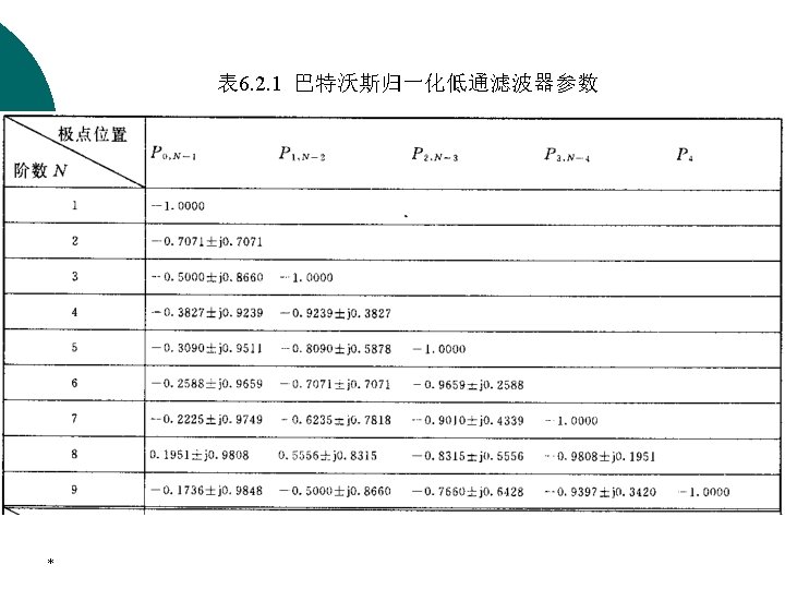
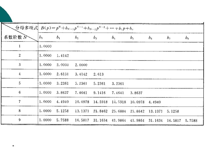
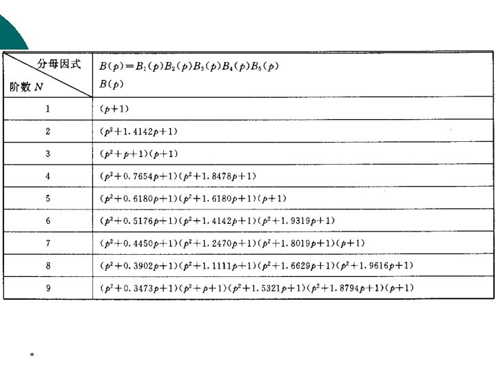
3. Butterwort approximation The expression for the transfer function of the Butterworth lowpass filter is given by where *

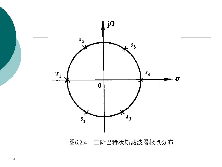
3. Butterwort approximation It can easily shown that p Poles are *

3. Butterwort approximation EXAMPLE 6. 2. 1 Design of Butterworth lowpass filter *

3. Butterwort approximation l Design of Butterworth lowpass filter with MATLAB [z, p, k]=buttap(k) [N, wc]=buttord(wp, ws, Rp, As, ‘s’) [B, A]=butter(N, wc, ‘ftype’, ‘s’) *

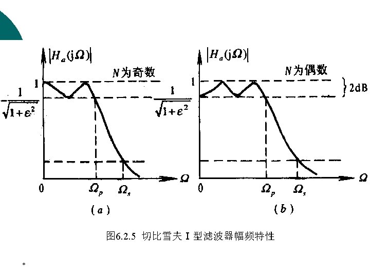
4. Chebychev approximation In this case, the approximation error, defined as the difference between the ideal brickwall characteristic and the actual response, is minimized over a prescribed band of frequencies. In fact, the magnitude error is equiripple in the band. *

4. Chebychev approximation l There are two types of Chebychev tranfser functions. In the Type 1 Chebyshev approximation, the magnitude characteristic is equiripple in the passband monotonic in the stopband, whereas in the Type 2 approximation, the magnitude response is monotonic in the passband equiripple in the stopband. *

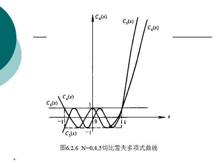
4. Chebychev approximation The magnitude-squared response of the analog lowpass Type 1 Chebychev filter of Nth order is given by Where 0<ε<1 is the ripple in the passband, CN is the Chebychev polynomial of order N. *

4. Chebychev approximation The above polynomial can also be derived via a recurrence relation given by With *

4. Chebychev approximation It can be seen that the squared-magnitude response is equiripple between x=0 and x=1, and it decreases monotonically for all x>1. *

4. Chebychev approximation The order N of the transfer function is determined from the attenuation specification in the stopband at a particular frequency. For example, if at = s, the magnitude is equal to the minimum stopband attenuation δs *

4. Chebychev approximation At , the magnitude is equal to the maximum passband attenuation , we can obtain Where We can also obtain *

4. Chebychev approximation At , the minimum stopband attenutation is obtained 由于 有 * , we can

4. Chebychev approximation We can obtain As in the case of the Butterworth filter, the order N of the filter is chosen as the nearest integer greater than or equal to the above number N. *

4. Chebychev approximation Further, at 3 db-cutoff-frequency, then We can also obtain *

4. Chebychev approximation The transfer function Ha(s) is a rational function *

4. Chebychev approximation At , the minimum stopband attenutation is obtained 可得 可得 * , we can

4. Chebychev approximation EXAMPLE 6. 2. 2 Design of Chebychev lowpass filter *

4. Chebychev approximation l Design of Chebychev filter using MATLAB [z, p, k]=cheb 1 ap(N, Rp) [N, wpo]=cheb 1 ord(wp, ws, Rp, As, ‘s’) [B, A]=cheby(N, Rp, wpo, ‘ftype’) [B, A]=cheby 1(N, Rp, wpo, ‘ftype’, ‘s’) *

4. Chebychev approximation Example 6. 2. 4 wp=2*pi*3000; ws=2*pi*12000; rp=0. 1; as=60; [N 1, wp 1]=cheb 1 ord(wp, ws, rp, as, ’s’); [B 1, A 1]=cheby 1(N 1, rp, wp 1, ’s’); Subplot(221); fk=0: 12000/512: 12000; wk=2*pi*fk; Hk=frqs(B 1, A 1, wk); Plot(fk/1000, 20*log 10(abs(Hk))); grid on *

5. Elliptic Approximation l 椭圆滤波器可以获得对理想滤波器幅频响应的最好逼 近，是一种性价比最高的滤波器。 l Since theory of elliptic filter approximation is mathematically quite involved, and a detailed treatment of this topic is beyond the scope of this text. *

5. Elliptic Approximation

5. Elliptic Approximation l 椭圆滤波器的MATLAB设计 【见教材P 169】 *

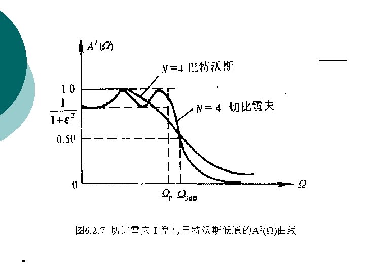
A Comparison of the Filter Types * ¡ Butterworth filter has the widest transition band, with a monotonically decreasing gain response. ¡ Another way of comparing the performances of the Butterworth, Chebyshev and elliptic filters would be compare the order of these filters required to meet the same filter specification.

6. Analog Highpass Filter Design ¡ * Two types of approximations dealt with the design of analog lowpass filters meeting the prescribed specifications have been discussed. Design of the other three classes of analog filters, namely, the highpass, bandpass, and bandstop filters, can be carried out by simple spectral transformations of the frequency variables.

6. Analog Highpass Filter Design l * Design Process of Analog Highpass Filter ¡ Development of the specifications of a prototype analog lowpass filter from the specifications of the desired analog highpass filter using a frequency transformation. ¡ Design of the analog prototype lowpass filter. ¡ Determination of the transfer function of the desired analog filter by applying the inverse of the frequency transformation used to determine the specifications of the prototype lowpass filter.

6. Analog Highpass Filter Design * ¡ The mapping from p-domain to s-domain is given by invertible p=F(s). ¡ The transfer functions Q(p) and Hd(s) are related through

6. Analog Highpass Filter Design ¡ A prototype analog lowpass transfer function Q(p) with a passband edge frequency p can be transformed into an analog highpass transfer function Hd(s) with a passband edge frequency ph using the spectral transformation On the imaginary axis, the above transformation reduces to *

6. Analog Highpass Filter Design ¡ The above mapping implies In passband In stopband *

6. Analog Highpass Filter Design ¡ * The above mapping ensures that the gain value of the prototype laowpass filter in its passband will appear in the passband of the desired highpass filter. Likewise, the gain value of the prototype lowpass filter in its stopband will appear in the stopband of the desired highpass filter.

6. Analog Highpass Filter Design ¡ * Example 6. 2. 5 P 172

6. Analog Highpass Filter Design % Exp 616. m Wp=1; ws=4; Rp=0. 1; As=40; [N, wc]=buttord(wp, ws, Rp, As, ‘s’) [B, A]=butter(N, wc, ’s’) Wph=2*pi*4000; [BH, AH]=lp 2 hp(B, A, wph) *

7. Analog Bandpass Filter Design ¡ The mapping relationship is On the imaginary axis, the above transformation reduces to *

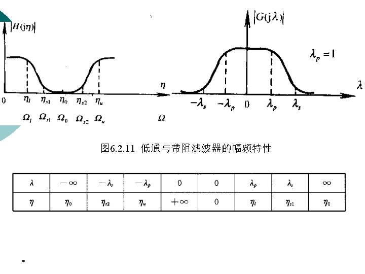
7. Analog Bandpass Filter Design The above mapping implies G(p) of lowpass filter in passband [-λp, λp] is mapped into H(s) of bandpass filter in passband. *

7. Analog Bandpass Filter Design Example 6. 2. 6 P 175 *

7. Analog Bandpass Filter Design MATLAB programm: Wp=2*pi*[4000, 7000]; Ws=2*pi*[2000, 9000]; Rp=1; As=20; [N, wc]=buttord(wp, ws, Rp, As, ’s’) [BB, AB]=butter(N, wc, ‘s’) *

8. Analog Bandstop Filter Design * ¡ The mapping relationship ¡ On the imaginary axis,

Transformation Method of IIR Filter Design ¡ A number of transformations have been proposed to convert an analog transfer function Ha(s) into a digital transfer function G(z) so that essential properties of the analog transfer function in s-domain are preserved for the digital transfer function in the z-domain. u Impulse Invariance Method u Bilinear Transformation Method *

6. 3 Impulse Invariance Method ¡ Definition The impulse response of the digital filter is identical to the impulse response of an analog prototype filter at sampling instants Let Ha(s) be analog transfer function, then The sample sequence of ha(t) is: *

6. 3 Impulse Invariance Method For single-poles case, namely We can be given by the inverse Laplace transform The discrete-time sequence can be given by sampling ha(t) with time interval T *

6. 3 Impulse Invariance Method We can obtain by Z transform Comparing H(z) with Ha(s), we can be given that the mapping relation between s-plane and z-plane is *

6. 3 Impulse Invariance Method Relation between s-plane and z-plane Let s=σ+j , z=rejω, we obtain *

6. 3 Impulse Invariance Method *

6. 3 Impulse Invariance Method *

6. 3 Impulse Invariance Method ¡ Due to sampling the mapping is many-toone ¡ The strips of length 2π/T are all mapped onto the unit circle ¡ Only if ha(t) is a band-limited signal, no alias will occur ¡ * Hence, this method is not suitable for highpass and bandstop filters design

6. 3 Impulse Invariance Method *

6. 3 Impulse Invariance Method *

6. 3 Impulse Invariance Method For a pair of conjugate-pole , namely We have *

6. 3 Impulse Invariance Method Advantage: p Linear frequency transformation 数字滤波器的单位脉冲响应完全模仿模拟滤波 器的单位冲激响应波形，时域特性逼近好。 p *

6. 3 Impulse Invariance Method Disadvantage: 若ha(t)频带不是限于±π/T之�，�会在奇数 π/T附近 产生频谱混叠。对应数字频率在ω =±π附近产生频谱 混叠。 ¡ * This method is not suitable for highpass and bandstop filters design.

6. 3 Impulse Invariance Method The impulse invariance transformation of an analog transfer function to digital transfer function can be carried out in MATLAB using the M-file impinvar. *

6. 3 Impulse Invariance Method * ¡ Example 6. 3. 1 the transfer function of a analog filter is ¡ Convert Ha(s) into the system function of the corresponding digital filter H(z) with impulse invariance method.

6. 4 The bilinear Transformation The bilinear transformation from the s-plane to the z-plane is given by It maps a single point in the s-plane to unique point in the z-plane. *

6. 4 Bilinear Transformation Method The relation between the digital transfer function G(z) and the parent analog transfer function Ha(s) is given by Step size The bilinear transformation is derived by applying the trapezoidal numerical integration approach to the differential equation representation of Ha(s) that leads to the difference equation representation of G(z). *

6. 4 Bilinear Transformation Method For Therefore *

6. 4 Bilinear Transformation Method It follows from the above equation that *

6. 4 Bilinear Transformation Method A point on the jΩ-axis in the s-plane (σ0=0) is mapped onto a point on the unit circle in the z-plane as |z|=1. A point in the left-half s-plane with σ0<0 is mapped onto a point inside the unit circle in the z-plane as |z|<1. A point in the rigth-half s-plane with σ0>0 is mapped onto a point outside the unit circle in the z-plane as |z|<1. *

6. 4 Bilinear Transformation Method The bilinear transformation mapping *

6. 4 Bilinear Transformation Method The exact relation between the imaginary axis in the splane and the unit circle in the z-plane *

6. 4 Bilinear Transformation Method Mapping of the angular analog frequencies to the angular digital frequencies ω via the bilinear transformation *

6. 3 Bilinear Transformation Method *

6. 4 Bilinear Transformation Method ¡ ¡ * It is clear that the mapping is highly nonlinear. This introduces a distortion in the frequency axis called frequency warping. The effect of warping is more evident in the below, which shows the transformation of a typical analog filter magnitude response to a digital filter magnitude response derived via the bilinear transformation.

6. 4 Bilinear Transformation Method *

6. 4 Bilinear Transformation Method To design a digital filter meeting the desired (digital) specifications we have to： ① We must first prewarp the critical bandedge frequencies to find their analog equivalent. ② Design the analog prototype Ha(s) using the prewarped critical frequencies. ③ Transform Ha(s) using the bilinear transformation to obtain the desired digital transfer function G(z). *

6. 4 Bilinear Transformation Method It should be noted that ¡ ü ü * the bilinear transformation preserves the magnitude response of an analog filter only if the specification requires piecewise constant magnitude. However, the phase response of the analog filter is not preserved after transformation。

6. 4 Bilinear Transformation Method ¡ * The bilinear transformation of an analog transfer function can be carried out in MATLAB using the M-file bilinear

6. 4 Bilinear Transformation Method ¡ We consider now the design of low-order digital filters by applying the bilinear transformation to the transfer functions of corresponding low-order analog filters. An application of these low-order digital filters are as equalizers in digital audio. ¡ *

6. 4 Bilinear Transformation Method ¡ * Example 6. 4. 1 Convert RC lowpass analog filter into the corresponding digital filter with the impulse invariance method and bilinear transformation method, respectively.

6. 4 Design of Lowpass IIR Digital Filters ¡ * We illustrate now the development of a lowpass IIR digital transfer function meeting given specifications using the bilinear transformation method.

6. 4 Bilinear Transformation Method l Design step of IIR digital lowpass filter based on the conversion of a prototype analog filter Determination of the digital lowpass filter specifications p Obtain the specifications for a prototype analog filter from the specifications of the desired digital filter p Design of the prototype analog filter p Convert the analog transfer function into digital transfer function p *

6. 4 Bilinear Transformation Method l First-order Butterworth lowpass digital filters The transfer function of a first-order Butterworth lowpass analog filter with 3 -d. Bcutoff frequency at Ωc is given by Applying the bilinear transformation, we arrive at the expression for transfer function G(z) of a first-order Butterworth digital lowpass filter: *

6. 4 Bilinear Transformation Method l * Example 6. 4. 2 P 187

6. 5 Design of Highpass, Bandpass and Bandstop Digital Filters ¡ The approach consists of the following steps: Step 1: Prewarp the specified digital frequency specifications of the desired digital filter GD(z) using Eq. (9. 18) to arrive at the frequency specifications of analog filter HD(s) of same type. Step 2: Convert the frequency specifications of HD(s) into those of a prototype analog lowpass filter HLP(s) using an appropriate frequency transformation. *

6. 5 Design of Highpass, Bandpass and Bandstop Digital Filters Step 3: Design the analog lowpass filter HLP(s). Step 4: Convert the transfer function HLP(s) into HD(s) using the inverse of the frequency transformation used in Step 2. Step 5: Transform the transfer function HD(s) using the bilinear transformation of Eq. (9. 14) to arrive at the desired digital IIR transfer function GD(z). *

6. 5 Design of Highpass, Bandpass and Bandstop Digital Filters Example 6. 5. 1 P 189 Example 6. 5. 2 P 191 *

6. 6 Spectral Transformations of IIR Filters * ¡ Often, in practice, it is necessary to modify the characteristics of a filter to meet the new specifications without repeating the filter design procedure. ¡ For example, after a lowpass filter with a password edge at 2 k. Hz has been designed, it may be required to move the passband edge to 2. 1 k. Hz.

6. 6 Spectral Transformations of IIR Filters ¡ * We describe here the spectral transformations that can be used to transform a given lowpass digital IIR transfer function GL(z) to another digital transfer function GD(z) that could be a lowpass, highpass, bandpass, or bandstop filter.

6. 6 Spectral Transformations of IIR Filters Spectral Transformation Using MATLAB ¡ * The M-files iirlp 2 lp, iirlp 2 hp, iirlp 2 bp and iirlp 2 bs can be used to carry out the desired spectral transforms.

6. 7 IIR digital filter design using MATLAB ¡ ¡ * The Signal Processing Toolbox of MATLAB includes a variety of M-files for the design of both IIR and FIR digital filters. We illustrate the use of some these functions in this section.

6. 7 IIR digital filter design using MATLAB ¡ The IIR digital filter design process involves two steps: ¡ Step 1: To determine the filter order N and the frequency scaling factor Wn from the given specifications. ¡ * Step 2: To determine the coefficients of the transfer function using the above parameters and the specified ripples.

6. 7 IIR digital filter design using MATLAB ¡ Order Estimation p buttord for the Butterworth filters p chebord for the Type 1 Chebyshev filters *

6. 7 IIR digital filter design using MATLAB ¡ Filter Design p butter for the design of Butterworth p cheby 1 for the design of Type 1 Chebyshev *

6. 7 IIR digital filter design using MATLAB ¡ Filter Design The output files could be either the numerator and denominator coefficient vectors or the vector of zeros, the vector of poles, and the scalar gain factor. *

6. 7 IIR digital filter design using MATLAB ¡ Filter Design The numerator and denominator coefficients of the transfer function can be determined from the latter data using the function zp 2 tf. The function zp 2 sos can be used to find the second-order factors of the numerator and the denominator of the transfer function. After the transfer function has been computed, the frequency response can be computed using the M-file freqz. *

6. 7 IIR digital filter design using MATLAB % Program 9_1 % Elliptic IIR Lowpass Filter Design % Wp = input('Normalized passband edge = '); Ws = input('Normalized stopband edge = '); Rp = input('Passband ripple in d. B = '); Rs = input('Minimum stopband attenuation in d. B = '); [N, Wn] = ellipord(Wp, Ws, Rp, Rs) [b, a] = ellip(N, Rp, Rs, Wn); [h, omega] = freqz(b, a, 256); plot (omega/pi, 20*log 10(abs(h))); grid; xlabel('omega/pi'); ylabel('Gain, d. B'); title('IIR Elliptic Lowpass Filter'); *

6. 7 IIR digital filter design using MATLAB % Program 9_2 % Type 1 Chebyshev IIR Highpass Filter Design % Wp = input('Normalized passband edge = '); Ws = input('Normalized stopband edge = '); Rp = input('Passband ripple in d. B = '); Rs = input('Minimum stopband attenuation in d. B = '); [N, Wn] = cheb 1 ord(Wp, Ws, Rp, Rs); [b, a] = cheby 1(N, Rp, Wn, 'high'); [h, omega] = freqz(b, a, 256); plot (omega/pi, 20*log 10(abs(h))); grid; xlabel('omega/pi'); ylabel('Gain, d. B'); title('Type I Chebyshev Highpass Filter'); *

6. 7 IIR digital filter design using MATLAB % Program 9_3 % Design of IIR Butterworth Bandpass Filter % Wp = input('Passband edge frequencies = '); Ws = input('Stopband edge frequencies = '); Rp = input('Passband ripple in d. B = '); Rs = input('Minimum stopband attenuation = '); [N, Wn] = buttord(Wp, Ws, Rp, Rs); [b, a] = butter(N, Wn); [h, omega] = freqz(b, a, 256); gain = 20*log 10(abs(h)); plot (omega/pi, gain); grid; xlabel('omega/pi'); ylabel('Gain, d. B'); title('IIR Butterworth Bandpass Filter'); *

6. 8 Computer-Aided Design of IIR Digital Filters ¡ The IIR digital filter design algorithms described in Sections 9. 2, 9. 4, and 9. 5 are based on the design of a prototype analog filter followed by its transformation to an IIR digital filter. These algorithms are used in applications requiring filters with a frequency-selective magnitude response with a lowpass, highpass, bandpass, or bandstop characteristics. n *

6. 8 Computer-Aided Design of IIR Digital Filters In applications requiring IIR digital filters with other types of frequency response, filter design algorithms rely on some type of iterative optimization techniques that are used to minimize the error between the desired frequency response and that of the computer-generated filter. n In this section, we first review the basic idea behind the computer-based iterative design techniques and then outline a specific application for the group delay equalization of IIR digital filters. n *

6. 8 Computer-Aided Design of IIR Digital Filters Let -- the frequency response of the digital transfer function H(z) to be designed. -- the desired frequency response, given as a piecewise linear function of ω, in some sense. *

6. 8 Computer-Aided Design of IIR Digital Filters The objective is for all values of ω over closed subintervals of 0<= ω<=π is minimized. is some user-specified positive weighting function. *

6. 8 Computer-Aided Design of IIR Digital Filters Some approximation measure The first approximation measure, called the Chebyshev or minimax criterion, is to minimize the peak absolute value of the weighted error The second approximation measure, called the leastp criterion, is to minimize the integral of pth power of the weighted error function *

6. 8 Computer-Aided Design of IIR Digital Filters In the case of IIR filter design, H(ejω) and D(ejω) are replaced with their magnitude functions. Moreover, the desired transfer function H(z) is assumed to be a real, rational function of z with fixed orders of the numerator and the denominator polynomials. The adjustable filter parameters are either the coefficients of the numerator and the denominator polynomials or the poles and zeros of the transfer function. The design objective is to iteratively adjust the filter parameters so that ε defined by either Eq. (9. 42) or Eq. (9. 44) is a minimum. *

6. 8 Computer-Aided Design of IIR Digital Filters ¡ ¡ ¡ * The IIR filter design methods described in Section 9. 2 through 9. 5 lead to transfer functions with nonlinear phase response resulting in group delays that are not constant in the passbands of the filters. To arrive at a frequency selective IIR digital filter with a constant group delay, a practical approach is to first design an IIR digital filter meeting the magnitude response specifications then design an allpass section. The allpass delay equalizer is usually designed using a computer-aided optimization method.

6. 8 Computer-Aided Design of IIR Digital Filters Let H(z) be the transfer function of IIR digital filter, with a group delay given by τH(ω). Our objective is to design a stable allpass section with a transfer function with a group delay τA(ω) so that the over group delay of the cascaded system is approximately constant in the passband of the filter. *