LINEARPHASE FIR FILTERS DESIGN Prof Siripong Potisuk FIR

LINEAR-PHASE FIR FILTERS DESIGN Prof. Siripong Potisuk

FIR Filter Characteristics l Completely specified by input-output relation: l bk = filter coefficients and M +1 = filter length All poles are at the origin always stable Impulse response has only a finite number of terms finite length l l

Group Delay l Negative of the slope of the phase response of a linear system, i. e. , filters l The amount by which the spectral component at frequency f gets delayed as it is processed by the filter A digital linear-phase filter has a constant group delay except possibly at frequencies at which the magnitude response is zero l

Generalized Linear-phase Filters where Ar( ) = Amplitude Response of H( ), = phase offset, and = group delay

Generalized Linear-phase Filters This is the necessary condition for h[n] to have linear phase. Two possible cases: (even symmetry) (odd symmetry)

Types of Linear-phase FIR filters Filter h[n] Filter Phase End-point type symmetry order offset zeros Candidate filters 1 Even 0 None All 2 Even Odd 0 z = 1 LP, BP 3 Odd Even /2 z = 1 BP 4 Odd /2 z=1 HP, BP

Impulse Responses of Four Types of FIR Linear-phase Filters

Linear-phase Zeros l l l l Symmetry condition imposes constraints on the zeros of a linear-phase FIR filter Transfer function satisfies: Type 1: no restriction on end-point zeros Type 2: an end-point zero at z = -1 Type 3: end-point zeros at z = 1 Type 4: an end-point zero at z = 1 All types: complex zeros in groups of four (r 1)

Pole-zero Plot of a Sixth-order, Type-1 Linear-phase FIR Filter

Example Construct a type 1 linear-phase filter of order 2 with Coefficients satisfying |bk| =1, k. Also, find the transfer function and its zeros.

Example Construct a type 2 linear-phase filter of order 1 with Coefficients satisfying |bk| =1, k. Also, find the transfer function and its zeros.

Example Construct a type 3 linear-phase filter of order 2 with Coefficients satisfying |bk| =1, k. Also, find the transfer function and its zeros.

Example Construct a type 4 linear-phase filter of order 1 with Coefficients satisfying |bk| =1, k. Also, find the transfer function and its zeros.

The Windowing Method l l l Start with the desired or ideal frequency response with appropriate delay Compute IDTFT to obtain the desired impulse response according the filter type & order Truncate the resulting impulse response using one of the finite-length windowing functions, i. e. , Rectangular, Bartlett, Hamming, Hanning, and Blackman

Ideal Lowpass Characteristics

Impulse Responses of Ideal Linear-phase type-1 FIR filters of Order M = 2 Filter type Lowpass Highpass Bandstop h[n], 0 k M, k h[ ]

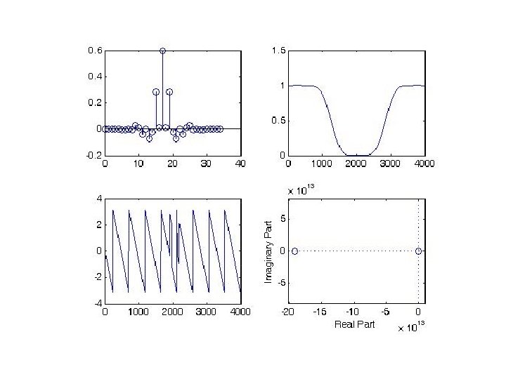
Example Construct a type 1 linear-phase filter of order 6 with coefficients satisfying the highpass response characteristics and cutoff frequency of 2000 Hz assuming a sampling frequency of 8000 Hz. Also, find the transfer function and generate the polezero plot. Repeat for order 40.

Windowing (Truncation) Effect 1. Passband & Stopband ripples caused by sidelobes 2. Transition bandwidth dependent on mainlobe width

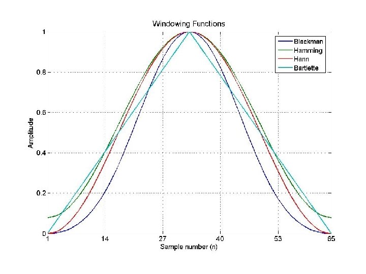
Commonly-used Windowing Functions

Effects of Window Shape & Size l l For a fixed size window, window shape affects both the mainlobe width and sidelobe height Window size affects the mainlobe width only

Green = Hamming Red = Hanning Teal = Blackman Blue = Rectangular

Meeting Design Specifications • Appropriate window selected based on frequencydomain specifications • Estimate the filter order, M, to control the width of the normalized transition band of the filter.

MATLAB Implementation l Function B = firwd(N, Ftype, WL, WH, Wtype) l MATLAB user-defined function for FIR filter design using the windowing method (text, pp. 288 -290) l Input Arguments: N = number of filter taps (must be an odd number) = M+1 where M is a filter order (even number for Type 1) Ftype = filter type ( 1 – lowpass, 2 – highpass, 3 – Bandpass, 4 – bandstop ) WL = lower cut-off frequency in rad (set to zero for highpass) WH = upper cutoff frequency in rad (set to zero for lowpass) Wtype = window type ( 1 – rectangular, 2 – triangular, 3 – Hanning, 4 – Hamming, 5 – Blackman )

Design Characteristics of Windows Passband Ripple Stopband Attenuation Window Type Filter Order (M) p Ap (d. B) s As (d. B) Rectangular 0. 9/ F 0. 0819 0. 7416 0. 0819 21 Hanning 3. 1/ F 0. 0063 0. 0546 0. 0063 44 Hamming 3. 3/ F 0. 0022 0. 0194 0. 0022 53 Blackman 5. 5/ F 0. 00017 74

Example 7. 11 Design a type 1 linear-phase filter with coefficients satisfying bandstop response characteristics with the following specifications: Lower cutoff frequency of 1250 Hz Lower transition width of 1500 Hz Upper cutoff frequency of 2850 Hz Upper transition width of 1300 Hz Stopband attenuation of 60 d. B Passband ripple of 0. 02 d. B Sampling frequency of 8000 Hz.

Kaiser Window l Near-optimal window defined as l = M/2, and I 0( ) represents the zeroth-order modified Bessel function of the 1 st kind Two parameters: M +1 = filter length and = shape parameter l

Kaiser Window Characteristics

Design Method where P is the passband cutoff frequency T is the stopband cutoff frequency is the passband ripple and stopband attenuation