Machine Vision ENT 273 Image Filters Hema C

Machine Vision ENT 273 Image Filters Hema C. R. Lecture 5 Hema ENT 273 Lecture 5

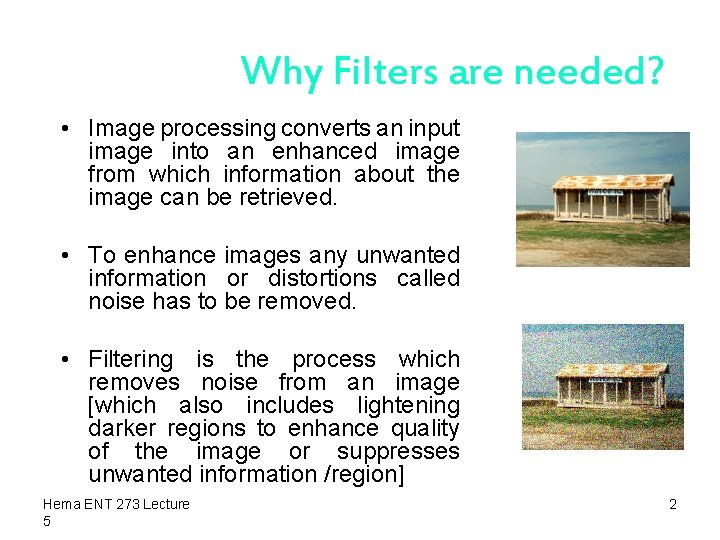
Why Filters are needed? • Image processing converts an input image into an enhanced image from which information about the image can be retrieved. • To enhance images any unwanted information or distortions called noise has to be removed. • Filtering is the process which removes noise from an image [which also includes lightening darker regions to enhance quality of the image or suppresses unwanted information /region] Hema ENT 273 Lecture 5 Original Image with Noise 2

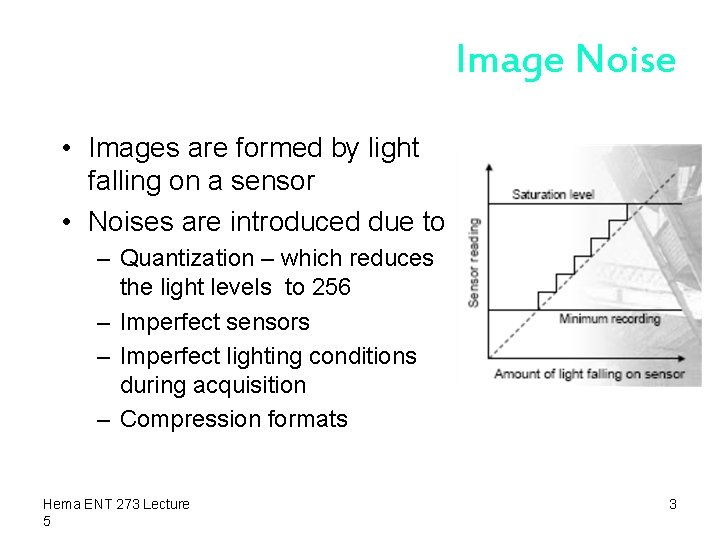
Image Noise • Images are formed by light falling on a sensor • Noises are introduced due to – Quantization – which reduces the light levels to 256 – Imperfect sensors – Imperfect lighting conditions during acquisition – Compression formats Hema ENT 273 Lecture 5 3

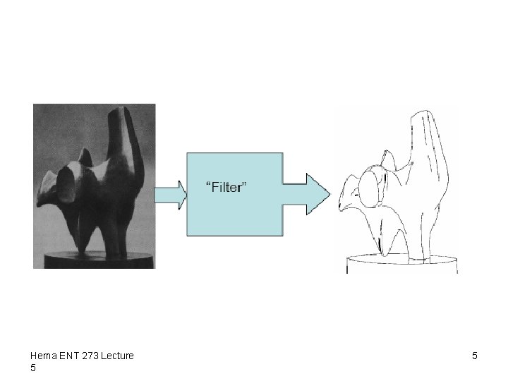
Features of Filter • Reduce the size of the data on which we want to build • our inferences • Reduction should retain most informative pieces – Edges and Corners – Texture • Mathematically/computationally Hema ENT 273 Lecture 5 4

Hema ENT 273 Lecture 5 5

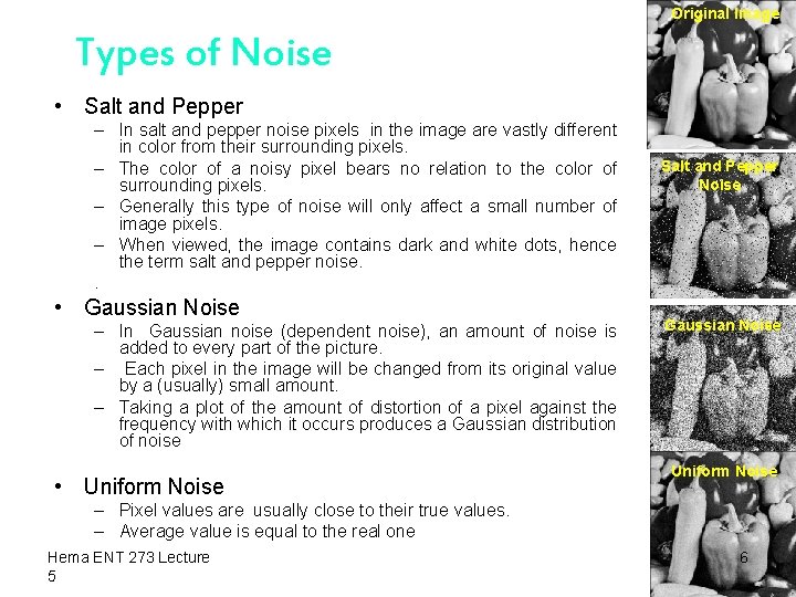
Original Image Types of Noise • Salt and Pepper – In salt and pepper noise pixels in the image are vastly different in color from their surrounding pixels. – The color of a noisy pixel bears no relation to the color of surrounding pixels. – Generally this type of noise will only affect a small number of image pixels. – When viewed, the image contains dark and white dots, hence the term salt and pepper noise. . • Gaussian Noise – In Gaussian noise (dependent noise), an amount of noise is added to every part of the picture. – Each pixel in the image will be changed from its original value by a (usually) small amount. – Taking a plot of the amount of distortion of a pixel against the frequency with which it occurs produces a Gaussian distribution of noise • Uniform Noise Salt and Pepper Noise Gaussian Noise Uniform Noise – Pixel values are usually close to their true values. – Average value is equal to the real one Hema ENT 273 Lecture 5 6

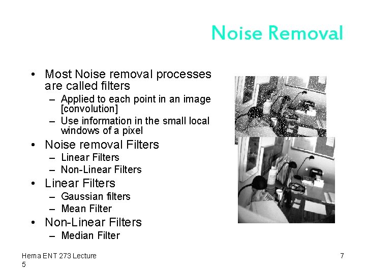
Noise Removal • Most Noise removal processes are called filters – Applied to each point in an image [convolution] – Use information in the small local windows of a pixel • Noise removal Filters – Linear Filters – Non-Linear Filters • Linear Filters – Gaussian filters – Mean Filter • Non-Linear Filters – Median Filter Hema ENT 273 Lecture 5 7

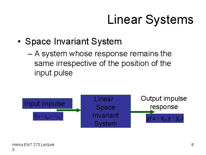
Linear Systems • Space Invariant System – A system whose response remains the same irrespective of the position of the input pulse Input impulse Hema ENT 273 Lecture 5 Linear Space Invariant System Output impulse response 8

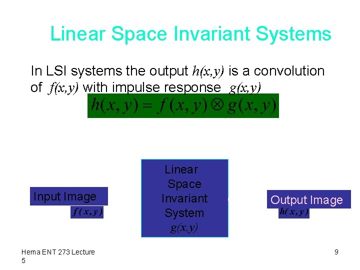
Linear Space Invariant Systems In LSI systems the output h(x, y) is a convolution of f(x, y) with impulse response g(x, y) Input Image Hema ENT 273 Lecture 5 Linear Space Invariant System g(x, y) Output Image 9

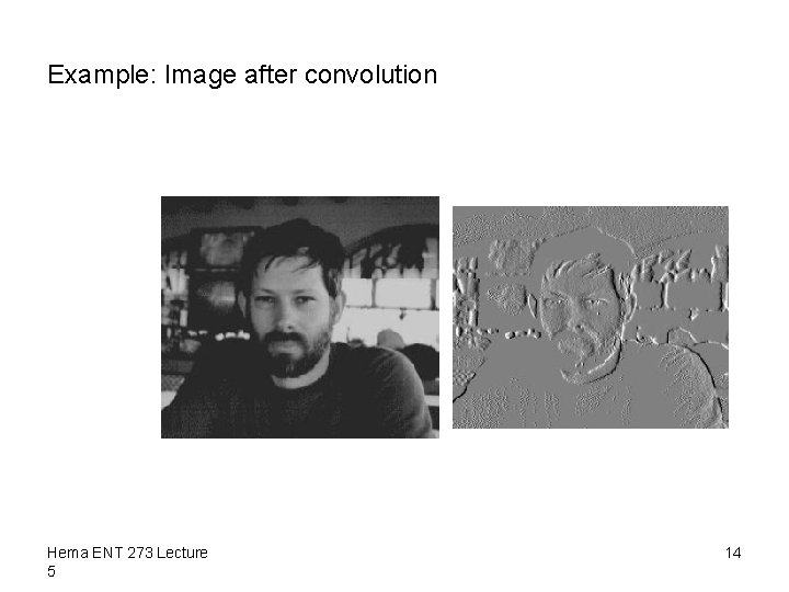
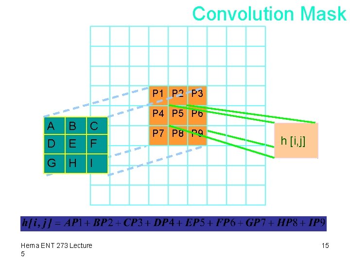
Convolution • Convolution – A neighborhood operation in which each output pixel is a weighted sum of neighboring input pixels. The weights are defined by the convolution kernel. Image processing operations implemented with convolution include smoothing, sharpening, and edge enhancement. – Convolution is a spatially invariant operation Hema ENT 273 Lecture 5 10

Convolution (cont. ) • One of the most important processes on images. • Actually a class of operations allowing much variety. • Used in almost all Computer Vision programs as a starting point. • Used in many Computer Graphics processes. Hema ENT 273 Lecture 5 11

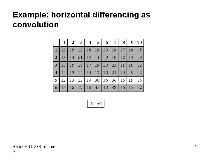
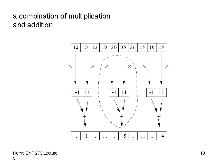
Example: horizontal differencing as convolution Hema ENT 273 Lecture 5 12

a combination of multiplication and addition Hema ENT 273 Lecture 5 13

Example: Image after convolution Hema ENT 273 Lecture 5 14

Convolution Mask P 1 P 2 P 3 P 4 P 5 P 6 A D B E C F G H I Hema ENT 273 Lecture 5 P 7 P 8 P 9 h [i, j] 15

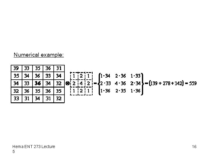
Hema ENT 273 Lecture 5 16

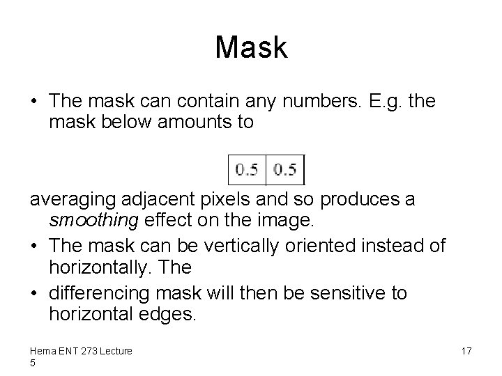
Mask • The mask can contain any numbers. E. g. the mask below amounts to averaging adjacent pixels and so produces a smoothing effect on the image. • The mask can be vertically oriented instead of horizontally. The • differencing mask will then be sensitive to horizontal edges. Hema ENT 273 Lecture 5 17

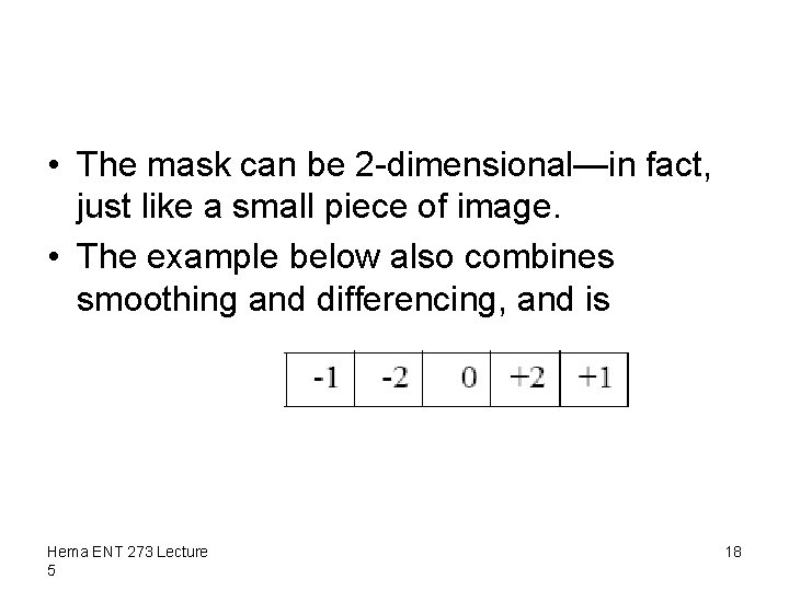
• The mask can be 2 -dimensional—in fact, just like a small piece of image. • The example below also combines smoothing and differencing, and is Hema ENT 273 Lecture 5 18

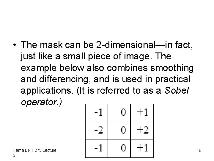
• The mask can be 2 -dimensional—in fact, just like a small piece of image. The example below also combines smoothing and differencing, and is used in practical applications. (It is referred to as a Sobel operator. ) Hema ENT 273 Lecture 5 19

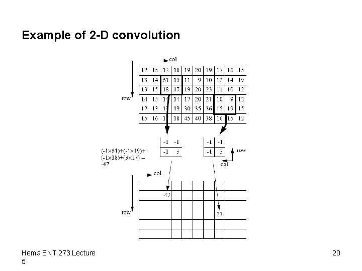
Example of 2 -D convolution Hema ENT 273 Lecture 5 20

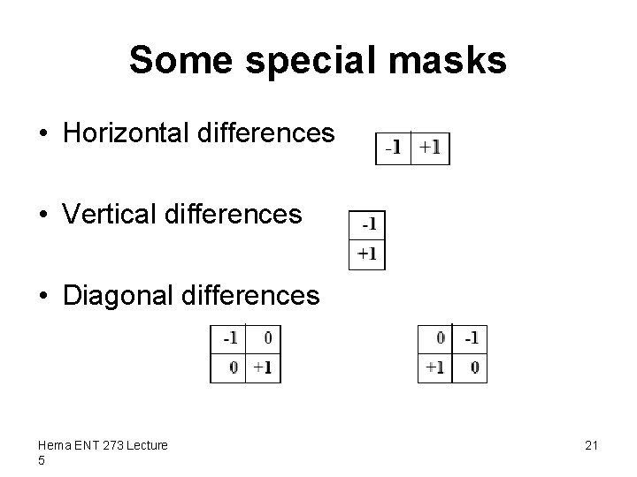
Some special masks • Horizontal differences • Vertical differences • Diagonal differences Hema ENT 273 Lecture 5 21

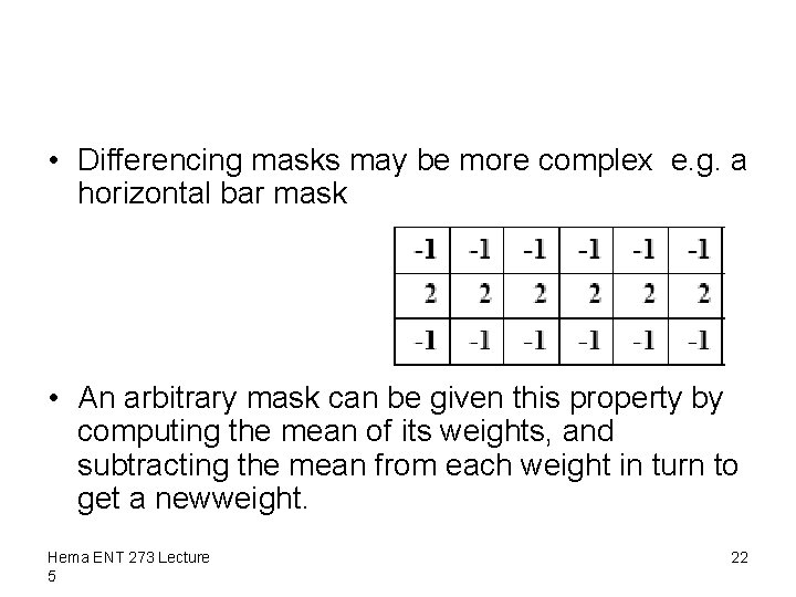
• Differencing masks may be more complex e. g. a horizontal bar mask • An arbitrary mask can be given this property by computing the mean of its weights, and subtracting the mean from each weight in turn to get a newweight. Hema ENT 273 Lecture 5 22

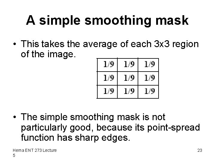
A simple smoothing mask • This takes the average of each 3 x 3 region of the image. • The simple smoothing mask is not particularly good, because its point-spread function has sharp edges. Hema ENT 273 Lecture 5 23

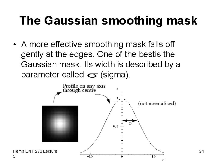
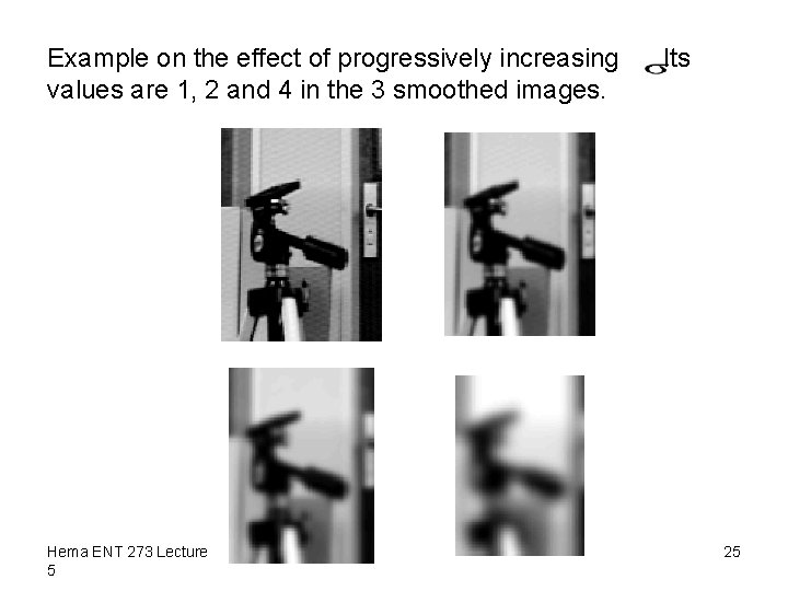
The Gaussian smoothing mask • A more effective smoothing mask falls off gently at the edges. One of the bestis the Gaussian mask. Its width is described by a parameter called (sigma). Hema ENT 273 Lecture 5 24

Example on the effect of progressively increasing values are 1, 2 and 4 in the 3 smoothed images. Hema ENT 273 Lecture 5 . Its 25

Feature of Linear Filter • About modifying pixels based on neighborhood. • Linear means linear combination of neighbors. – Linear methods simplest – Can combine linear methods in any order to achieve same result – Maybe easier to undo – “Filter Banks” Hema ENT 273 Lecture 5 26

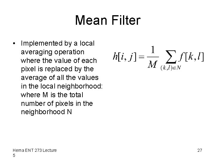
Mean Filter • Implemented by a local averaging operation where the value of each pixel is replaced by the average of all the values in the local neighborhood: where M is the total number of pixels in the neighborhood N Hema ENT 273 Lecture 5 27

• 3 x 3 neighborhood about [i, j] Hema ENT 273 Lecture 5 28

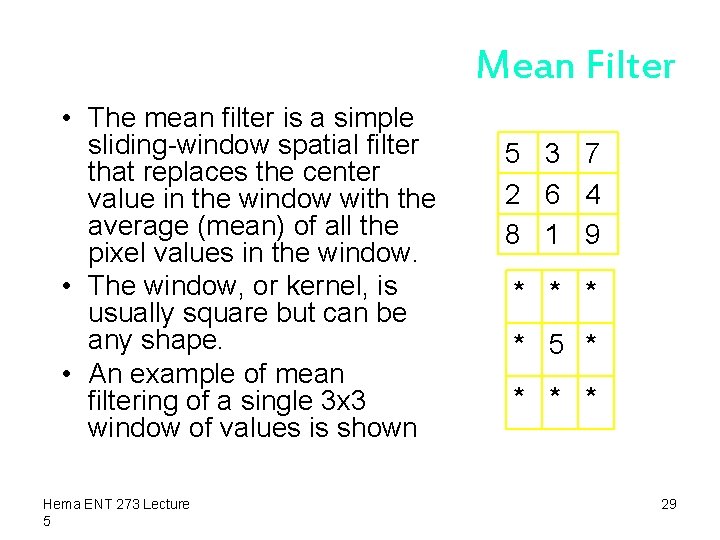
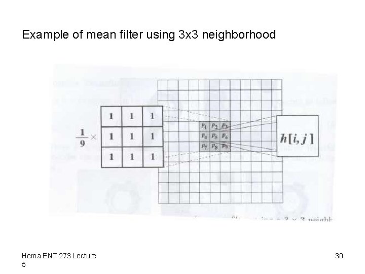
Mean Filter • The mean filter is a simple sliding-window spatial filter that replaces the center value in the window with the average (mean) of all the pixel values in the window. • The window, or kernel, is usually square but can be any shape. • An example of mean filtering of a single 3 x 3 window of values is shown Hema ENT 273 Lecture 5 5 3 7 2 6 4 8 1 9 * * 5 * * 29

Example of mean filter using 3 x 3 neighborhood Hema ENT 273 Lecture 5 30

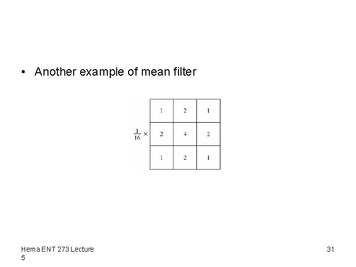
• Another example of mean filter Hema ENT 273 Lecture 5 31

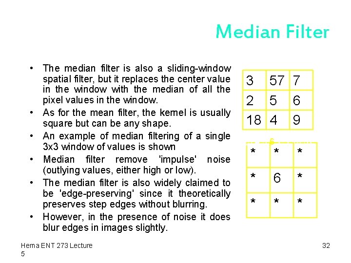
Median Filter • The median filter is also a sliding-window spatial filter, but it replaces the center value 3 57 7 in the window with the median of all the pixel values in the window. 2 5 6 • As for the mean filter, the kernel is usually 18 4 9 square but can be any shape. • An example of median filtering of a single 2, 3, 4, 5, 6, 7, 9, 18, 57 3 x 3 window of values is shown * * * • Median filter remove 'impulse' noise (outlying values, either high or low). * 6 * • The median filter is also widely claimed to be 'edge-preserving' since it theoretically preserves step edges without blurring. * * * • However, in the presence of noise it does blur edges in images slightly. Hema ENT 273 Lecture 5 32

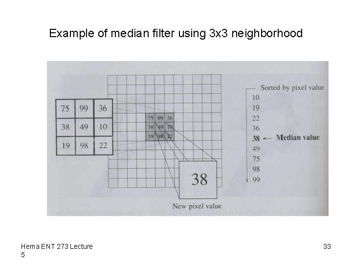
Example of median filter using 3 x 3 neighborhood Hema ENT 273 Lecture 5 33

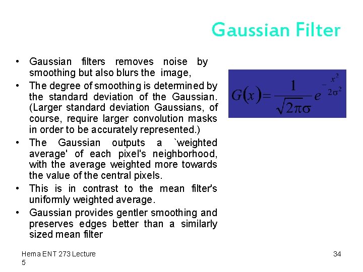
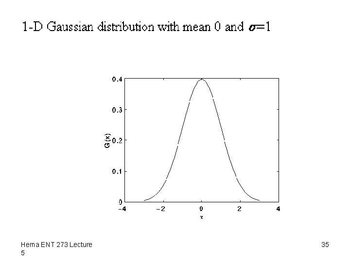
Gaussian Filter • Gaussian filters removes noise by smoothing but also blurs the image, • The degree of smoothing is determined by the standard deviation of the Gaussian. (Larger standard deviation Gaussians, of course, require larger convolution masks in order to be accurately represented. ) • The Gaussian outputs a `weighted average' of each pixel's neighborhood, with the average weighted more towards the value of the central pixels. • This is in contrast to the mean filter's uniformly weighted average. • Gaussian provides gentler smoothing and preserves edges better than a similarly sized mean filter Hema ENT 273 Lecture 5 34

Hema ENT 273 Lecture 5 35

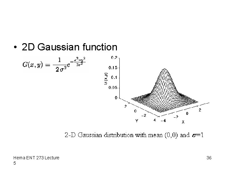
• 2 D Gaussian function Hema ENT 273 Lecture 5 36

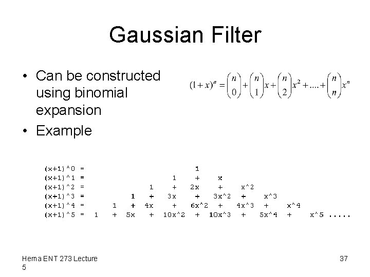
Gaussian Filter • Can be constructed using binomial expansion • Example Hema ENT 273 Lecture 5 37

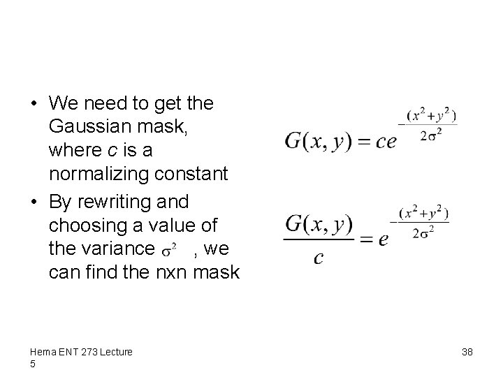
• We need to get the Gaussian mask, where c is a normalizing constant • By rewriting and choosing a value of the variance , we can find the nxn mask Hema ENT 273 Lecture 5 38

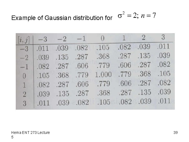
Example of Gaussian distribution for Hema ENT 273 Lecture 5 39

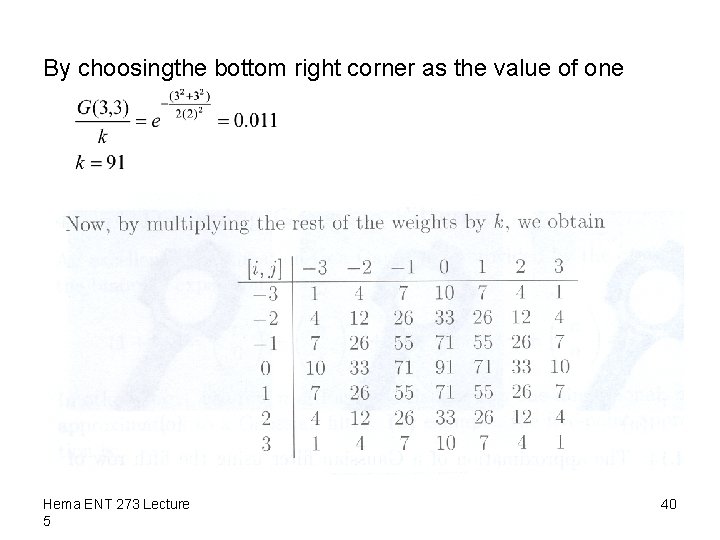
By choosingthe bottom right corner as the value of one Hema ENT 273 Lecture 5 40

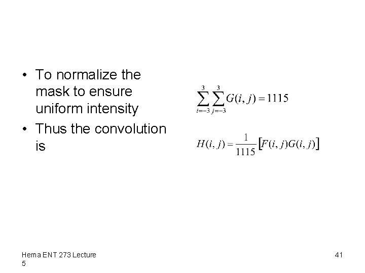
• To normalize the mask to ensure uniform intensity • Thus the convolution is Hema ENT 273 Lecture 5 41

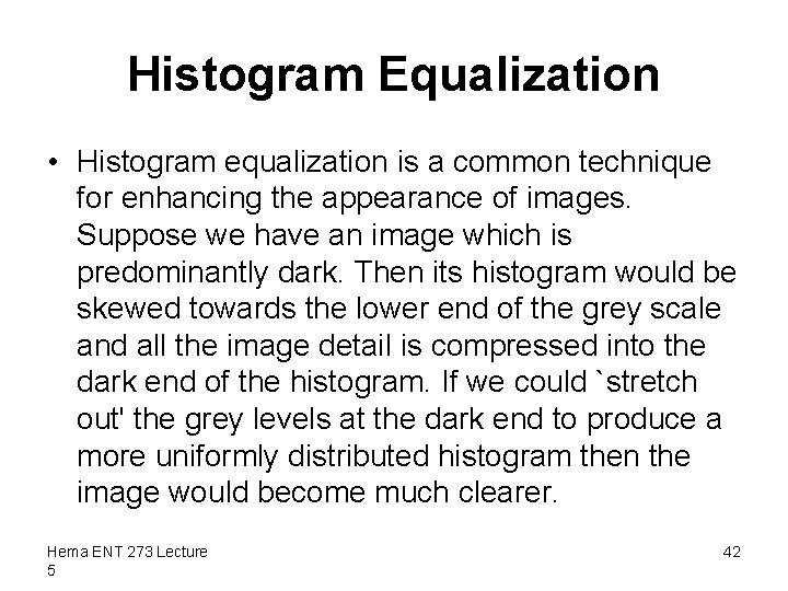
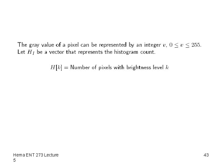
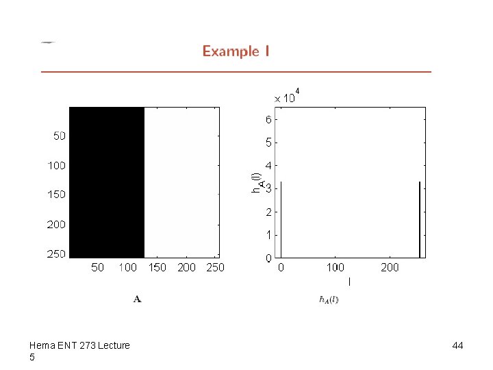
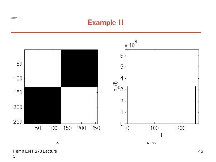
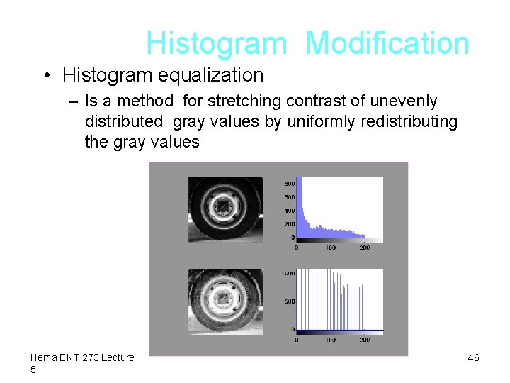
Histogram Equalization • Histogram equalization is a common technique for enhancing the appearance of images. Suppose we have an image which is predominantly dark. Then its histogram would be skewed towards the lower end of the grey scale and all the image detail is compressed into the dark end of the histogram. If we could `stretch out' the grey levels at the dark end to produce a more uniformly distributed histogram then the image would become much clearer. Hema ENT 273 Lecture 5 42

Hema ENT 273 Lecture 5 43

Hema ENT 273 Lecture 5 44

Hema ENT 273 Lecture 5 45

Histogram Modification • Histogram equalization – Is a method for stretching contrast of unevenly distributed gray values by uniformly redistributing the gray values Hema ENT 273 Lecture 5 46

References • Computer Vision – Linda G Shapiro & George Stockman • http: //en. wikipedia. org/wiki/Image_noise • Mat lab reference notes Hema ENT 273 Lecture 5 47

Machine Vision End of Lecture 5 Hema ENT 273 Lecture 5