Infinite Impulse Response Filters Presenteed By Dr M

Infinite Impulse Response Filters Presenteed By Dr M. Murugappan School of Mechatronic Engineering Universiti Malaysia Perlis

Introduction A digital filter is a linear time invariant (LTI) discrete time system. v The FIR and IIR filters are of type of non-recursive and recursive type, respectively. v In FIR filter design, the present output sample depends on the present and previous input samples. v In IIR filter design, the present output sample depends on the present, past and output samples. v The Impulse response for realizable filter and The stability condition must satisfy. v v The IIR digital filters have the transfer function form

Analog vs. Digital Filters Analog • • Speed 10 -100 x faster Dynamic Range Amplitude: 140 d. B e. g. , 12 Vrms & 1 � V noise – Frequency: 8 decades e. g. , 0. 01 Hz to 1 MHz – • • Cheap, small, low power Precision limited by noise & component tolerances Digital • • Very complex filters Full adjustability Precision vs. cost Arbitrary magnitude Total linear phase EMI & magnetic noise immunity Stability (temp & time) Repeatability

Frequency Selective Filters q q A filter rejects the unwanted frequencies from the input signal and allow the desired frequencies. The ranges frequencies that passed the filter is called the passband those which are blocked called stopband. The filter are of different types. v Lowpass Filter v Highpass Filter v Bandreject Filter

Design of Digital Filters from Analog Filters 1. 2. 3. The most common technique used for designing IIR digital filters known as Indirect Method. The derivation of digital filter transfer function required 3 steps: Map desired digital filter specifications into equivalent analog filter. Derive analog transfer function for the analog prototype. Transform the transfer function of the analog prototype into equivalent digital filter transfer function. Specification for the magnitude response of low pass filter (a)analog (b)digital (c) Alternate specifications of magnitude response of a lowpass filter

n n Fig (b) can be modified to apply to analog lowpass filter as in Fig (a). Here the digital frequencies ωp, ωs and ωc are replaced by analog frequencies Ωp, Ωs, and Ωc whose unit in radians/sec. Analog Filter Digital filter Process analog input and generates analog output. Process and generates digital data Constructed from active or passive electronic components. Consist of elements: adder, multiplier and delay unit. The frequency response modified by changing the components. The frequency response changed by changing the filter coefficient. Described using differential equation. Described by difference equation. Disadvantage: Quantization error arises due to finite length of the representation of signals and parameters.

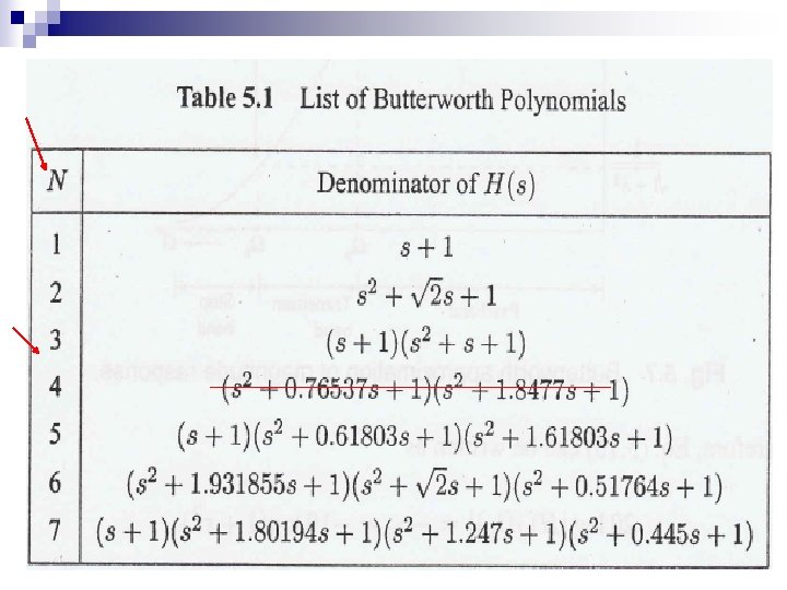
Analog Lowpass Filter Design General form analog filter transfer function is: Where H(s) is the Laplace transform of the impulse response h(t), N M must satisfied and H(s) must lie in left half of the s-plane. Analog lowpass Butterworth filter Magnitude function of Butterworth lowpass filter is given by N=order of the filter =cutoff frequency Seen, magnitude of response approaches ideal low pass characteristic as order N inc.

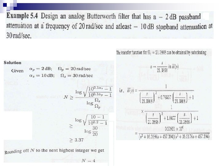
Round N to the close integer, get N=4

Determine the order and the poles of low pass Butterworth filter that has 3 d. B attenuation at 500 Hz and attenuation of 40 d. B at 1000 Hz. Round N = 7 Steps to design Analog Butterworth lowpass Filter v v v From given specifications, find order of the filter, N. Round off it to the next higher integer. Find the transfer function H(s) for Ωc =1 rad/sec for the value of N Calculate value of cutoff frequency, Ωc. Find the transfer function Ha (S) for value Ωc by substituting s -> s/ Ωc in H(s).

Analog Frequency Transformations Convert to Lowpass with cutoff 0 Highpass with cutoff 0 Bandpass with cutoffs 1 and 2 Bandstop with cutoffs 1 and 2 Replace s with

Design of IIR filters from analog filters The conversion technique should be effective it should posses following desirable properties. v The jΩ –axis in the s-plane should map into the unit circle in the zplane. Thus, have direct relationship between two frequency variable in two domain. v The left–half plane of the s-plane should map into the inside of the unit circle in the z-plane. Thus, we can convert stable analog to stable digital filter. 4 most widely use Methods for digitizing Analog filter to digital filter • Approximation of derivatives. • Impulse invariant transformation. • Bilinear transformation. • matched z-transformation technique.

Design of IIR Filter using Impulse Invariance Technique IIR filter is design such that unit impulse response h(n) of digital filter is the sampled version of the impulse response of analog filter. The z-transform of infinite impulse response given by Let us consider the mapping points from the s-plane to the z-plane by the relation z=es. T. Substitute s=σ+jΩ and express the complex variable z in polar form: z=rejω = e(σ+jΩ)T , we r = eσT, ω = ΩT. Therefore, analog is mapped to a place in the z plane of magnitude eσT and angle ΩT

Real part of analog pole =radius zplane, Imaginary part=angle of digital pole, Consider any pole on jΩ -axis, where σ=0. Poles maps at the z-plane at a radius r=e 0. T=1. Therefore, the impulse invariance had map poles from the splane’s jΩ -axis to z-plane’s unit circle. 2 nd case Consider pole on left–half s-plane where σ < 0. Therefore, all s-plane poles with negative real parts map to z-plane poles inside the unit circle – stable analog poles are mapped to stable digital poles. Because r= eσT<1 for <0.

Unstable pole mapping occur when all poles at right half of the s-plane map to the digital poles outside the unit circle. Third case many point in s-plane are mapped in one point in z-plane. Easiest way to explain is to consider two poles in the s=plane with identical real parts. n S 1= , S 2= Impulse invariant pole mapping

These pole map to z-plane poles z 1 and z 2, via impulse invariant mapping. Let Ha(s) is the system function of an analog filter and {ck} are the coefficients and {pk} are the poles of analog filter. The inverse laplace transform of Ha(s) Sampled ha(t) periodically at t=n. T ,

For high sampling rates (small T), the digital gain is high, we can use

Step to design a digital filter using impulse invariance method v For given specifications, find Ha(s), transfer function of analog filter. Select sampling rate of the digital filter, T second per sample. Express analog transfer function as sum of single-pole filters. v Compute the z-transform of the digital filter using formula v For high sampling rates v v

For the analog transfer function determine H(z) using impulse invariance method. Ass T=1 sec.

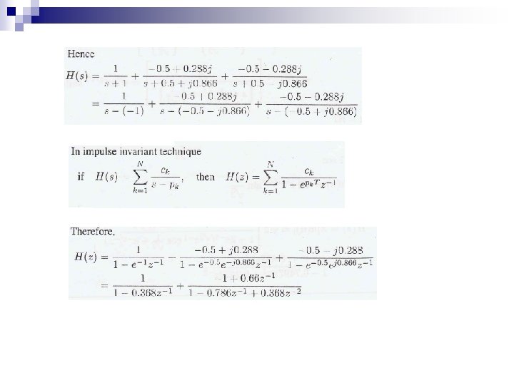
Design third order Butterworth digital filter using impulse invariant technique. Ass sampling period T=1 sec.

Design of IIR filter using Bilinear Transformation It is a conformal mapping that transforms the jΩ –axis into unit circle in the z-plane only once, that avoid aliasing components. q All point in LHP ‘s’ mapped inside unit circle z-plane. q All points in RHP ’s’ mapped outside unit circle z-plane. Let consider analog linear filter with system function q Which an be written Can be characterize by differential equation Approximate by trapeizoidal formula y’(t) is derivative of y(t)

Approximation of the integral at t=n. T and t 0=n. T-T yield From differential eq Which implies

The system function of the digital filter is Dividing numerator and Denominator by Relation between s ad z known as Bilinear transformation. Let z=rejw.

. Separating imaginary and real parts

Steps to Design Digital filter using Bilinear Transform technique 1. From the given specifications, find prewarping analog frequencies using formula 2. Using the analog frequencies, find H(s) of analog filter 3. Select the sampling rate of the digital filter, call T seconds per sample. 4. Substitute into the transfer function found in step 2. .

Apply Bilinear Tansformation to H(s)= with T=1 sec and find H(z).

Using the Bilinear transformation, design a highpass filter, monotonoic in passband with cutoff frequency 1000 Hz and down 10 d. B at 350 Hz. The sampling frequency is 5000 Hz. Therefore we take N =1. The 1 st order Butterworth filter for From Fig 5. 27, Prewarping the digital frequencies we have

Determine H(z) that result when the bilinear transformation is applied to Ha(s)= Solution: In bilinear transformation Ass T= 1 sec. Then, .

Realization of Digital Filters There are two type of realization of digital filter transfer function. Recursive Realization Non-Recursive Realization The current output y(n) is a Current output sample y(n) is a function of past outputs, past function of only past and present inputs. Correspond to IIR digital filter. Correspond to FIR digital filter.

IIR Filter can be realized in many forms v Direct form -I realization v Direct form –II realization v Transposed direct form realization v Cascade form realization v Parallel form realization v Lattice form realization.

Direct Form 1 realization Let consider an LTI recursive system describe by difference equation n. Structure call n. Direct form 1

Realize the second order digital filter y(n) =

Direct form II realization Consider the difference equation and from which The system of above difference equation The equation 5. 112 and Eq 5. 113 b can be expressed in difference equation form Which gives

n The realization Eq. (5. 114) and Eq. (5. 115) shown in Fig. (5. 35) , (5. 36)

Realize the second order system y(n) n we realize eq. (5. 118 a) and n and eq. (5. 118 b) n

Determine the direct form II realization for the following system . n The solution the system function given Realize eq. (5. 120) and n eq. (5. 121) and combine them n to get direct II realization of the n system shown below n Let,

Cascade Form n Let consider IIR System with system Function n Represented using block diagram n Realize each Hk(z) in direct form II and cascade all structure

Realizing H 1(z) and H 2(z)in direct form II, and cascading we obtain cascade form of system function.

Realize the system with difference equation y(n) = ¾ y(n-1)1/8 y(n-2)+x(n) +1/3 x(n-1) in cascade form. Solution , n From the difference equation H 1(z) can be realize in direct form II, >Similarly, H 2(z) can be realize n Direct form II Cascading the realization of H 1(z) and H 2(z)

Analog Lowpass Chebyshev Filters There are 2 types of Chebyshev filters n Type – I They are all-pole filters that exhibit equiripple behaviour in the passband a monotonic characteristics in the stopband. n Type – II Contains both poles and zeros and exhibits a monotonic behaviour in the passband equiripple behaviour in the stopband. n The magnitude square response of Nth order type I filter Where ε is a parameter of the filter related to the ripple in the passband CN(x) is the Nth order Chebyshev polynominal

Pole locations for Chebyshev Filter

Comparison between Butterworth and Chebyshev Filter n n n The magnitude response of Butterworth filter decreases monotonically as the frequency Ω increases from 0 to ∞, whereas the magnitude response of the Chebyshev filter exhibits ripples in the passband or stopband according to the type. The transition band is more in Butterworth filter when compared to Chebyshev filter. The poles of the Butterworth filter lie on a circle, whereas the poles of the Chebyshev filter lie on the ellipse. Steps to design an analog Chebyshev lowpass filter 1. From the given specifications, find the order of the filter N. 2. Round off it to the next higher integer. 3. Using the following formulas find the values of a and b, which are minor and major axis of the ellipse respectively.

4. Calculate the poles of Chebyshev filter which lie on the ellipse by using the formula 5. Find the denominator polynomial of the transfer function using above poles. The numerator of the transfer function depends on the value of N. (a) For N odd substitute s = 0 in the denominator polynomial and find the value. This value is equal to the numerator of the transfer function. (b) For N even substitute s = 0 in the numerator polynomial and divide the result by √ 1+ε 2. This value is equal to the numerator. 6.

Determine the order and the poles of a type I lowpass Chebyshev filter that has a 1 d. B ripple in the passband frequency Ωp = 1000π, a stopband frequency of 2000π and an attenuation of 40 d. B or more. Given data: αp = 1 d. B, Ωp = 1000π, αs = 40 d. B, Ωp = 2000π N= 5

Given the specifications αp = 3 d. B ; αs = 16 d. B ; fp = 1 k. Hz, and fs = 2 k. Hz, Determine the order of the filter using Chebyshev approximation. Find H(s). From the given data we can find, Ωp = 2π x 1000 = 2000 π rad/sec Ωs = 2π x 2000 = 4000 π rad/sec Step 1: Find N Step 2: Rounding N to next higher value we get N = 2 Step 3: The values of minor axis and major axis can be found as below x+jy

n. The denominator of H(s) = (s+643. 46π)2 +(1554π)2 (s+x)2+(y)2 n. The numerator of H(s) =(643. 46π)2 +(1554π)2/√ 1+ε 2 (x)2+(y)2 / √ 1+ε 2 =(1414. 38)2π2 The transfer function H(s) = (1414. 38)2π2/ (s 2+1287πs+(1682)2π2 Design a Chebyshev low pass filter with the specifications αp = 1 d. B ripple in the passband 0 ≤ ω ≤ 0. 2π, αs = 15 d. B ripple in the stopband 0. 3π ≤ ω ≤ π, using (a), bilinear transformation, (b). Impulse invariance. Given data αp = 1 d. B ; ωp = 0. 2π, αs = 15 d. B; ωs = 0. 3π Prewarped frequencies are given by

The denominator of H(s) =[(s+0. 0907)2 +(0. 639)2] [(s+0. 2189)2 +(0. 2647)2] =(s 2+0. 1814 s+0. 4165) (s 2+0. 4378 s+0. 118) As N is even, the numerator of H(s) =(0. 4165) (0. 118)/√ 1+ε 2 =0. 04381 The transfer function H(s) = 0. 04381/[(s 2+0. 1814 s+0. 4165) (s 2+0. 4378 s+0. 118)]

H(z) = H(s) | Impulse Invariance Method: Given data αp = 1 d. B ; ωp = 0. 2π, αs = 15 d. B; ωs = 0. 3π

The denominator of H(s) =[(s+0. 0876)2 +(0. 619)2] [(s+0. 2115)2 +(0. 2564)2] =(s 2+0. 175 s+0. 391) (s 2+0. 423 s+0. 11) As N is even, the numerator of H(s) =(0. 391) (0. 11)/√ 1+ε 2 =0. 03834 The transfer function H(s) = 0. 03834 / [(s 2+0. 175 s+0. 391) (s 2+0. 423 s+0. 11)] H(s) Using Impulse invariant transform

HOME WORK n FREQUENCY TRANSFORMATION BASED IIR FILTER DESIGN

THANK YOU ALL THE BEST