Digital Filters Analog Filters Digital Filters Cheap Costly

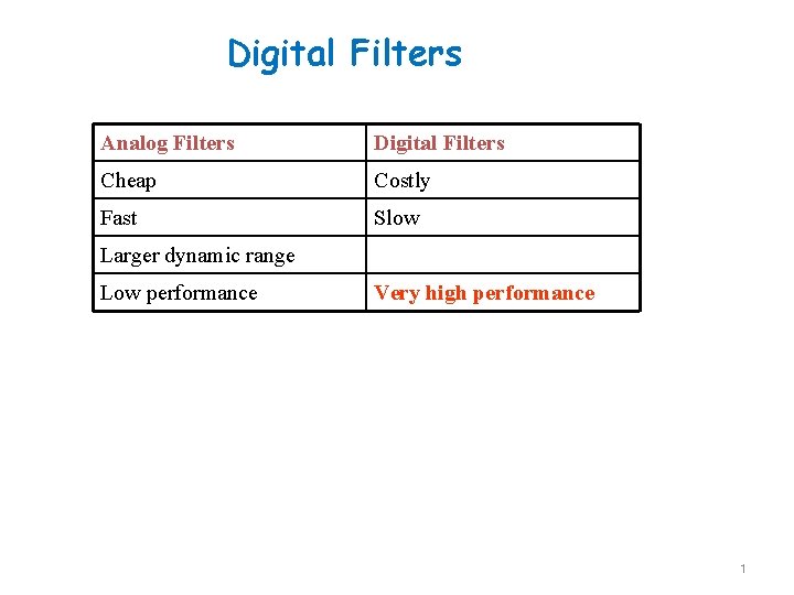
Digital Filters Analog Filters Digital Filters Cheap Costly Fast Slow Larger dynamic range Low performance Very high performance 1

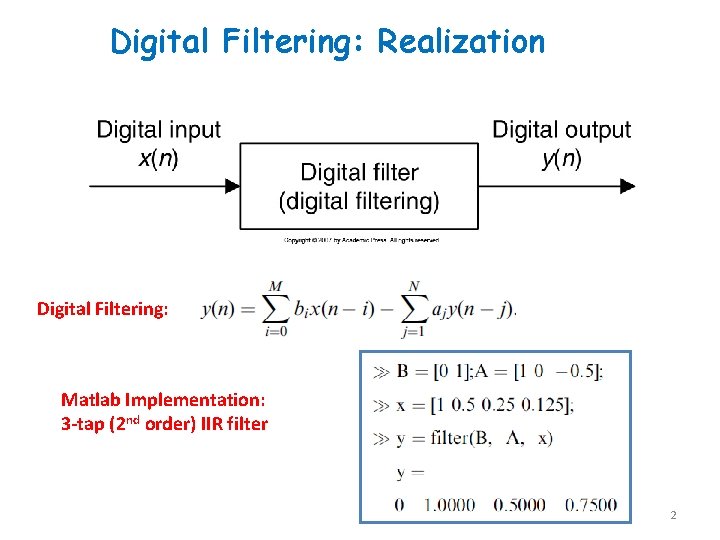
Digital Filtering: Realization Digital Filtering: Matlab Implementation: 3 -tap (2 nd order) IIR filter 2

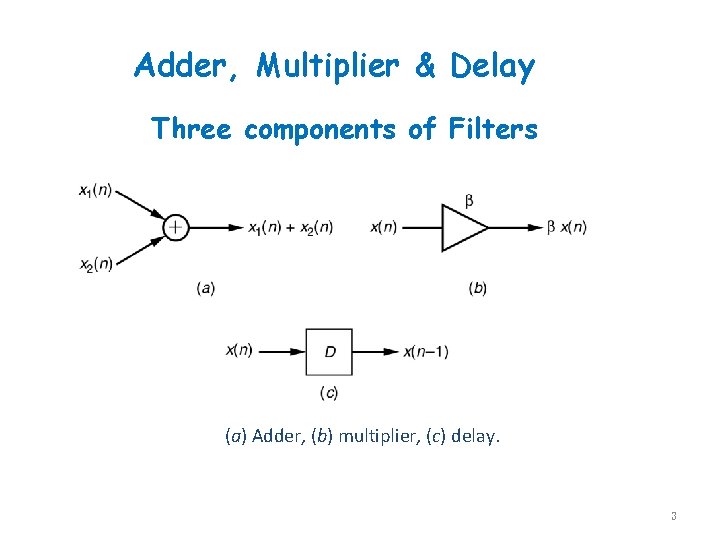
Adder, Multiplier & Delay Three components of Filters (a) Adder, (b) multiplier, (c) delay. 3

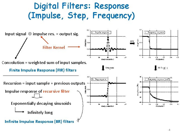
Digital Filters: Response (Impulse, Step, Frequency) Input signal impulse res. = output sig. Filter Kernel Convolution = weighted sum of input samples. Finite Impulse Response (FIR) filters Recursion = input sample + previous outputs Impulse response of recursive filter Exponentially decaying sinusoids Infinitely long Infinite Impulse Response (IIR) filters 4

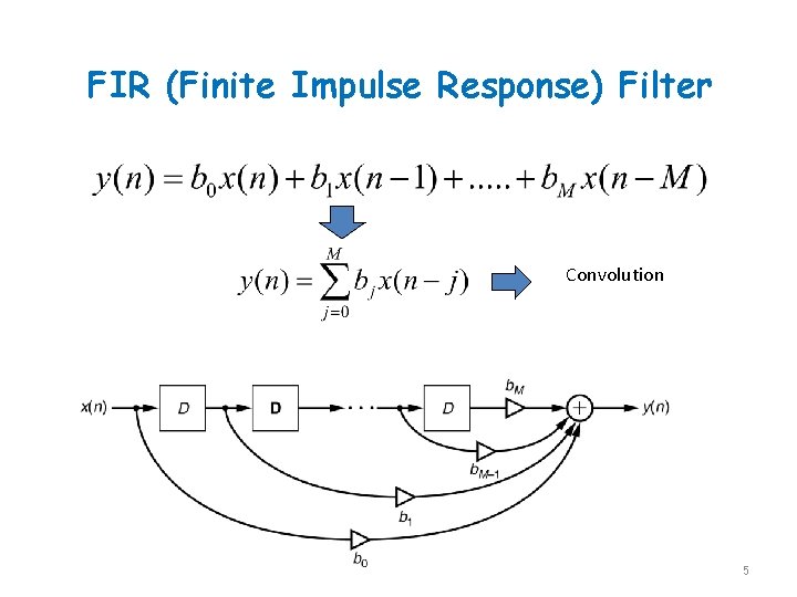
FIR (Finite Impulse Response) Filter Convolution 5

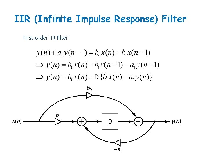
IIR (Infinite Impulse Response) Filter First-order IIR filter. 6

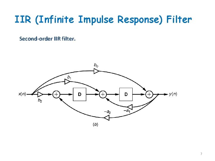
IIR (Infinite Impulse Response) Filter Second-order IIR filter. 7

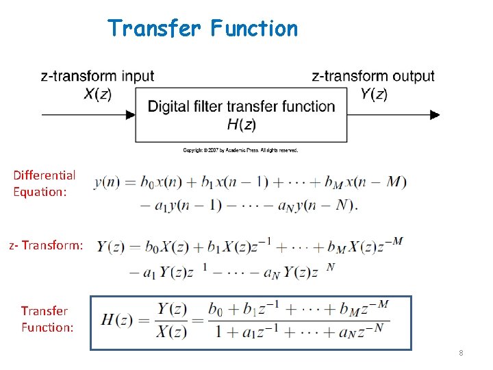
Transfer Function Differential Equation: z- Transform: Transfer Function: 8

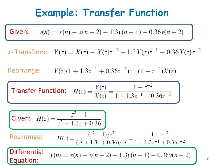
Example: Transfer Function Given: z- Transform: Rearrange: Transfer Function: Given: Rearrange: Differential Equation: 9

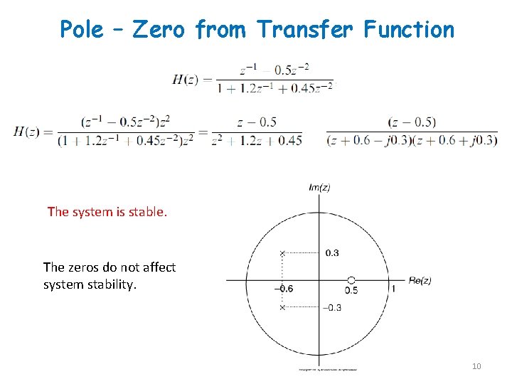
Pole – Zero from Transfer Function The system is stable. The zeros do not affect system stability. 10

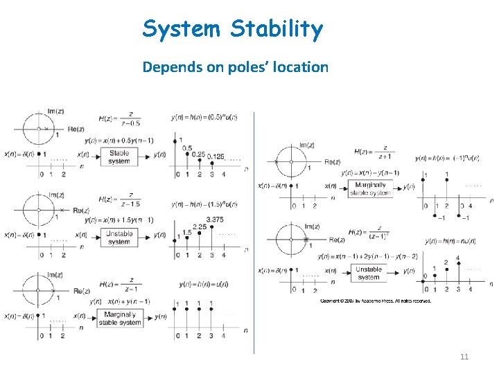
System Stability Depends on poles’ location 11

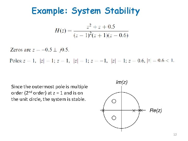
Example: System Stability Since the outermost pole is multiple order (2 nd order) at z = 1 and is on the unit circle, the system is stable. 12

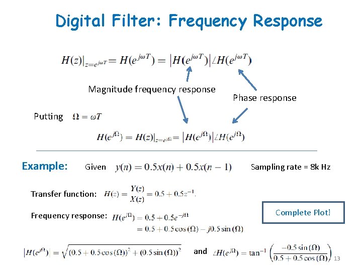
Digital Filter: Frequency Response Magnitude frequency response Phase response Putting Example: Given Sampling rate = 8 k Hz Transfer function: Complete Plot! Frequency response: and 13

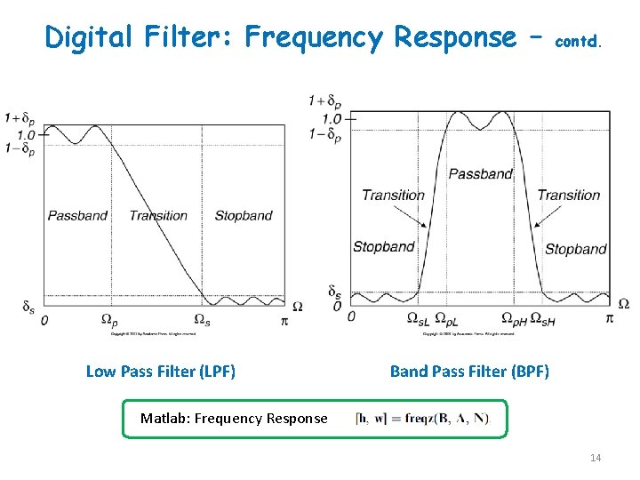
Digital Filter: Frequency Response – Low Pass Filter (LPF) contd. Band Pass Filter (BPF) Matlab: Frequency Response 14

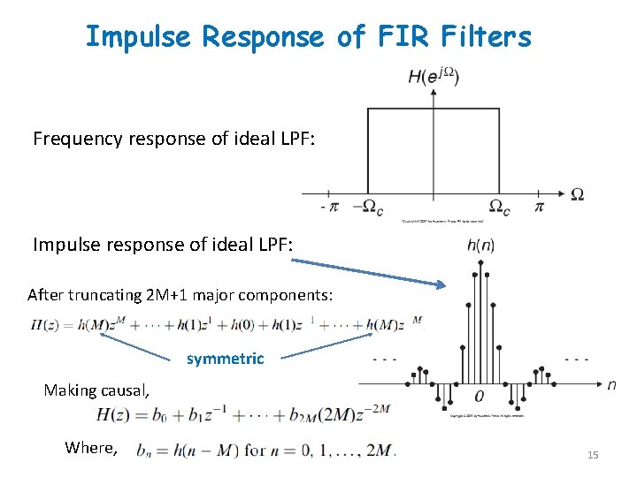
Impulse Response of FIR Filters Frequency response of ideal LPF: Impulse response of ideal LPF: After truncating 2 M+1 major components: symmetric Making causal, Where, 15

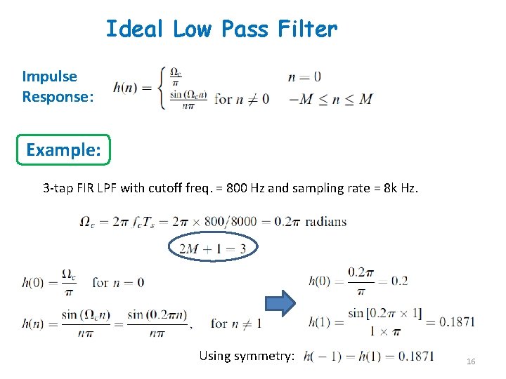
Ideal Low Pass Filter Impulse Response: Example: 3 -tap FIR LPF with cutoff freq. = 800 Hz and sampling rate = 8 k Hz. Using symmetry: 16

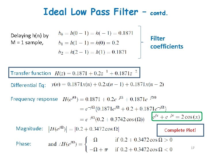
Ideal Low Pass Filter – Delaying h(n) by M = 1 sample, contd. Filter coefficients Transfer function Differential Eq: Frequency response Magnitude: Phase: Complete Plot! 17

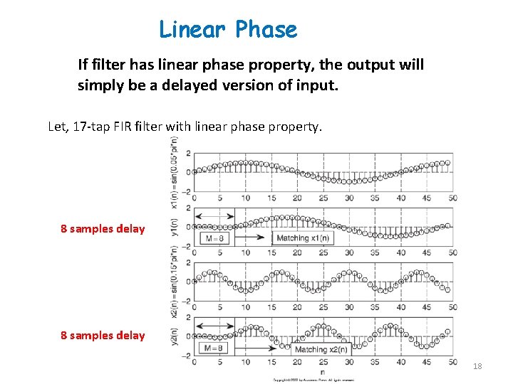
Linear Phase If filter has linear phase property, the output will simply be a delayed version of input. Let, 17 -tap FIR filter with linear phase property. 8 samples delay 18

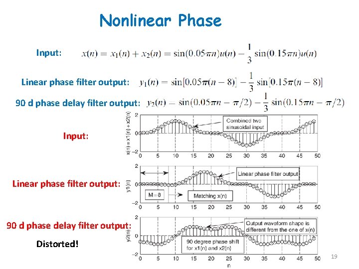
Nonlinear Phase Input: Linear phase filter output: 90 d phase delay filter output: Input: Linear phase filter output: 90 d phase delay filter output: Distorted! 19

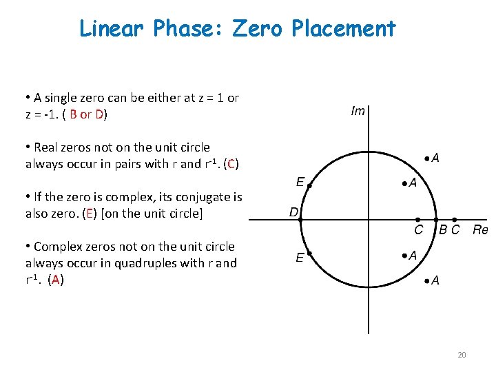
Linear Phase: Zero Placement • A single zero can be either at z = 1 or z = -1. ( B or D) • Real zeros not on the unit circle always occur in pairs with r and r-1. (C) • If the zero is complex, its conjugate is also zero. (E) [on the unit circle] • Complex zeros not on the unit circle always occur in quadruples with r and r-1. (A) 20

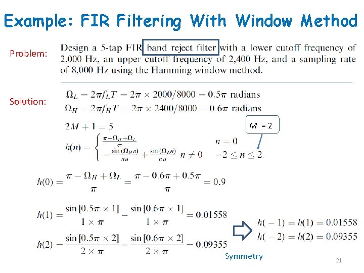
Example: FIR Filtering With Window Method Problem: Solution: M =2 Symmetry 21

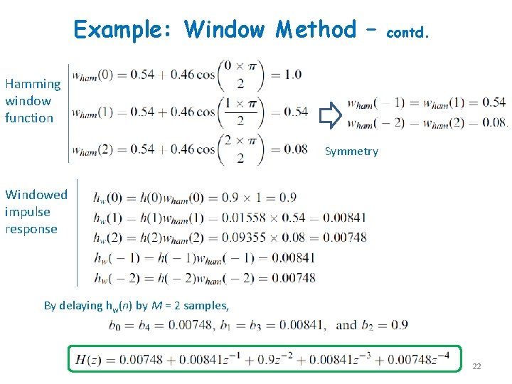
Example: Window Method – contd. Hamming window function Symmetry Windowed impulse response By delaying hw(n) by M = 2 samples, 22

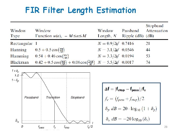
FIR Filter Length Estimation 23

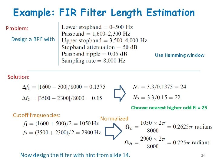
Example: FIR Filter Length Estimation Problem: Design a BPF with Use Hamming window Solution: Choose nearest higher odd N = 25 Cutoff frequencies: Normalized Now design the filter with hint from slide 14. 24

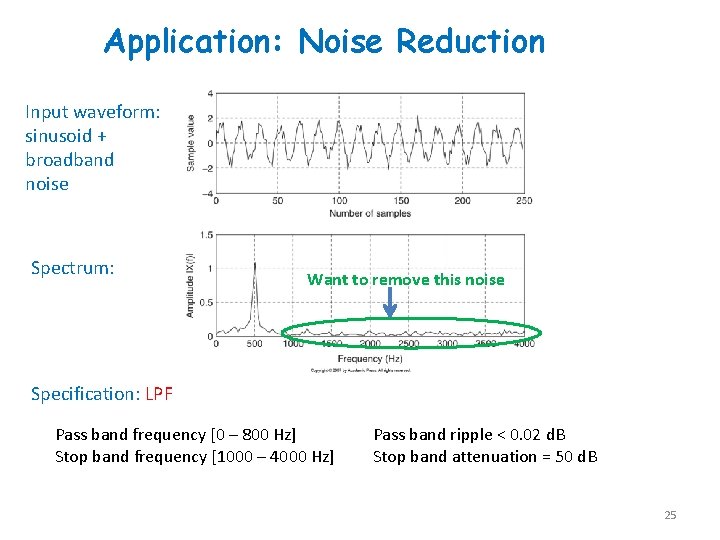
Application: Noise Reduction Input waveform: sinusoid + broadband noise Spectrum: Want to remove this noise Specification: LPF Pass band frequency [0 – 800 Hz] Stop band frequency [1000 – 4000 Hz] Pass band ripple < 0. 02 d. B Stop band attenuation = 50 d. B 25

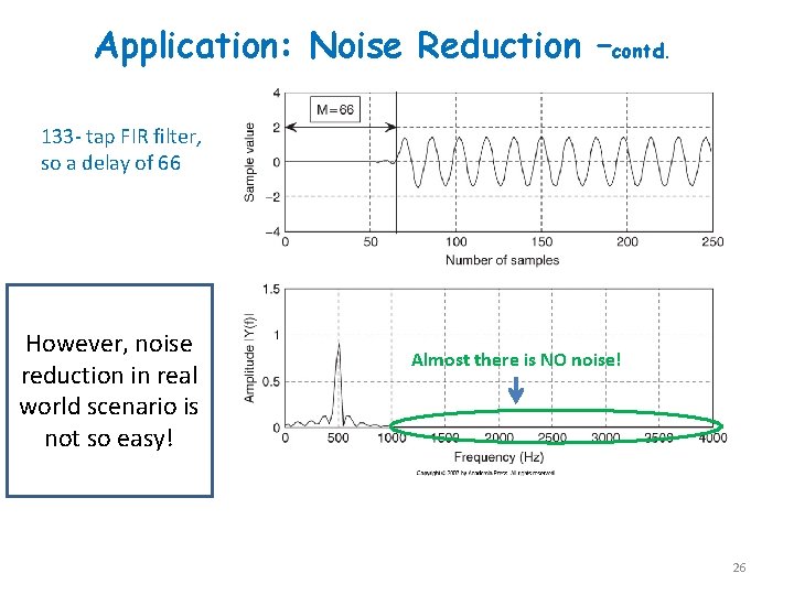
Application: Noise Reduction –contd. 133 - tap FIR filter, so a delay of 66 However, noise reduction in real world scenario is not so easy! Almost there is NO noise! 26

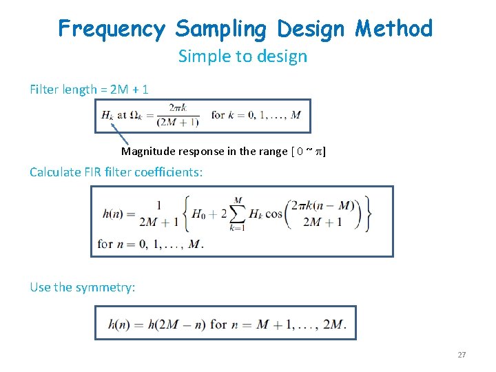
Frequency Sampling Design Method Simple to design Filter length = 2 M + 1 Magnitude response in the range [ 0 ~ ] Calculate FIR filter coefficients: Use the symmetry: 27

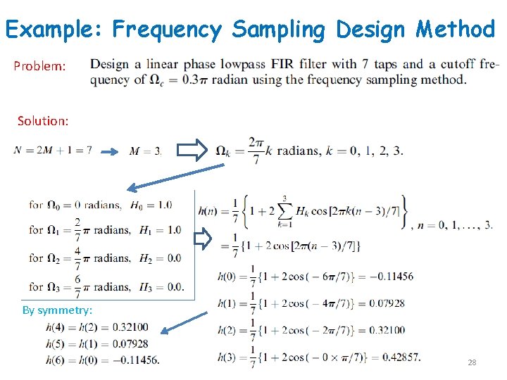
Example: Frequency Sampling Design Method Problem: Solution: By symmetry: 28

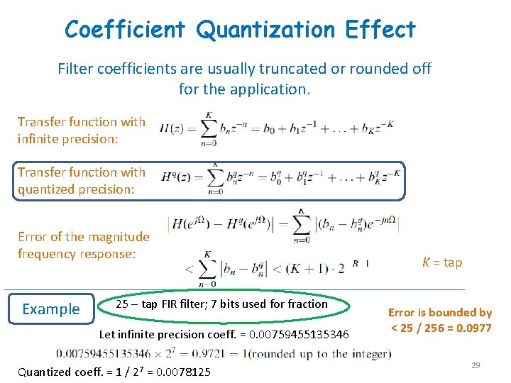
Coefficient Quantization Effect Filter coefficients are usually truncated or rounded off for the application. Transfer function with infinite precision: Transfer function with quantized precision: Error of the magnitude frequency response: Example 25 – tap FIR filter; 7 bits used for fraction Let infinite precision coeff. = 0. 00759455135346 Quantized coeff. = 1 / 27 = 0. 0078125 K = tap Error is bounded by < 25 / 256 = 0. 0977 29

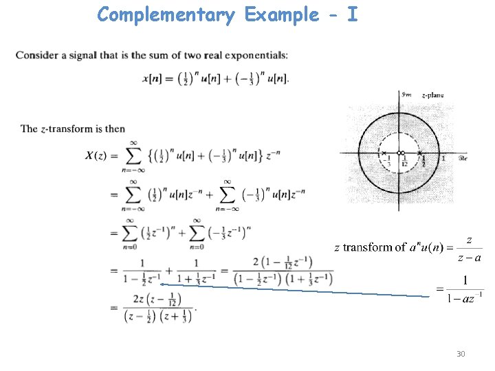
Complementary Example - I 30

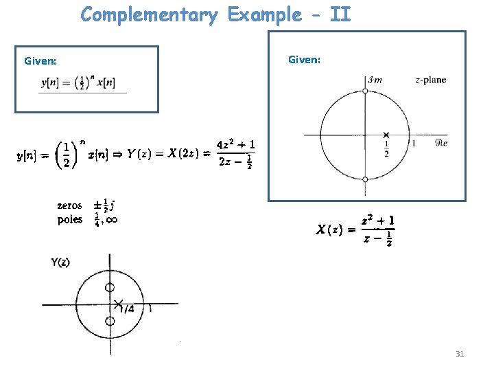
Complementary Example - II Given: 31

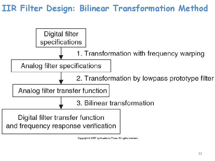
IIR Filter Design: Bilinear Transformation Method 32

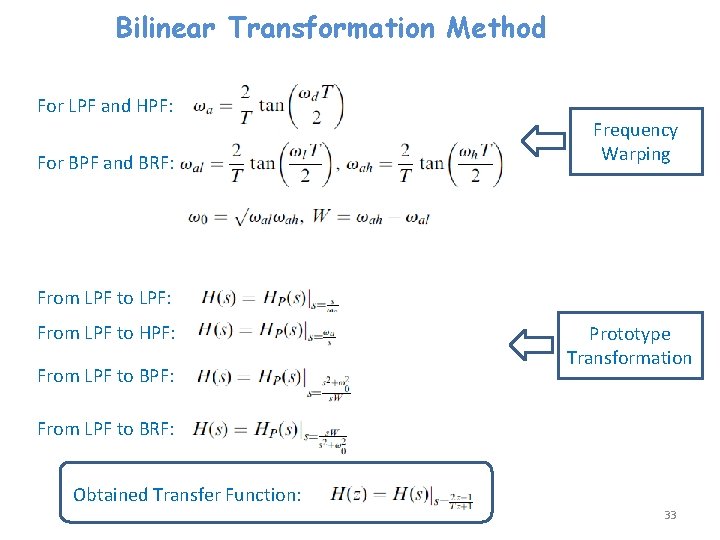
Bilinear Transformation Method For LPF and HPF: For BPF and BRF: Frequency Warping From LPF to LPF: From LPF to HPF: From LPF to BPF: Prototype Transformation From LPF to BRF: Obtained Transfer Function: 33

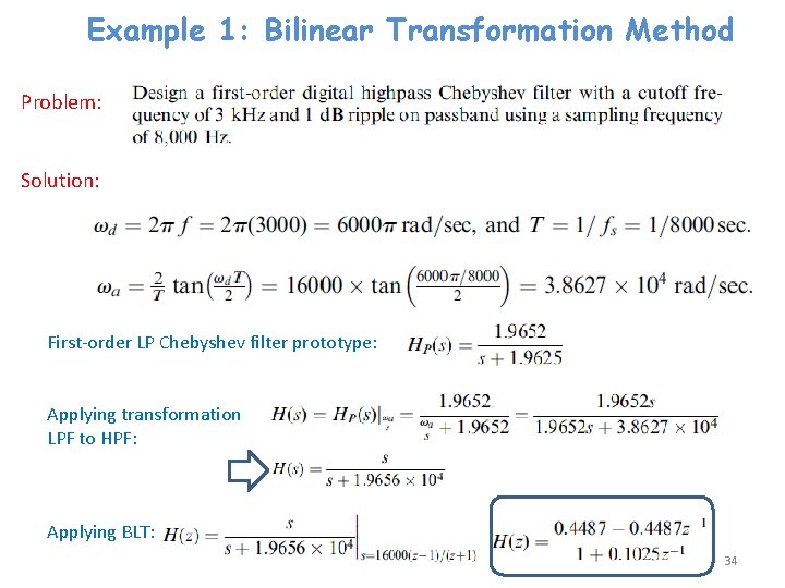
Example 1: Bilinear Transformation Method Problem: Solution: First-order LP Chebyshev filter prototype: Applying transformation LPF to HPF: Applying BLT: 34

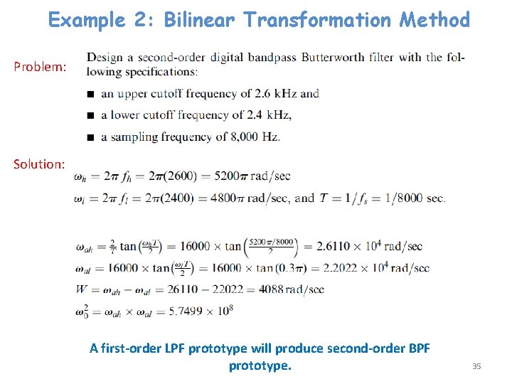
Example 2: Bilinear Transformation Method Problem: Solution: A first-order LPF prototype will produce second-order BPF prototype. 35

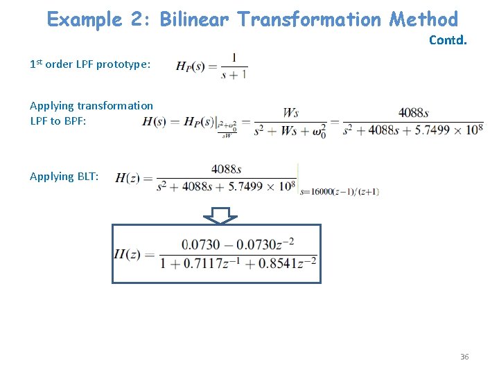
Example 2: Bilinear Transformation Method Contd. 1 st order LPF prototype: Applying transformation LPF to BPF: Applying BLT: 36

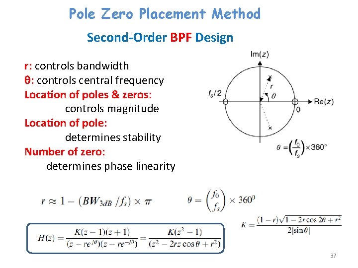
Pole Zero Placement Method Second-Order BPF Design r: controls bandwidth : controls central frequency Location of poles & zeros: controls magnitude Location of pole: determines stability Number of zero: determines phase linearity 37

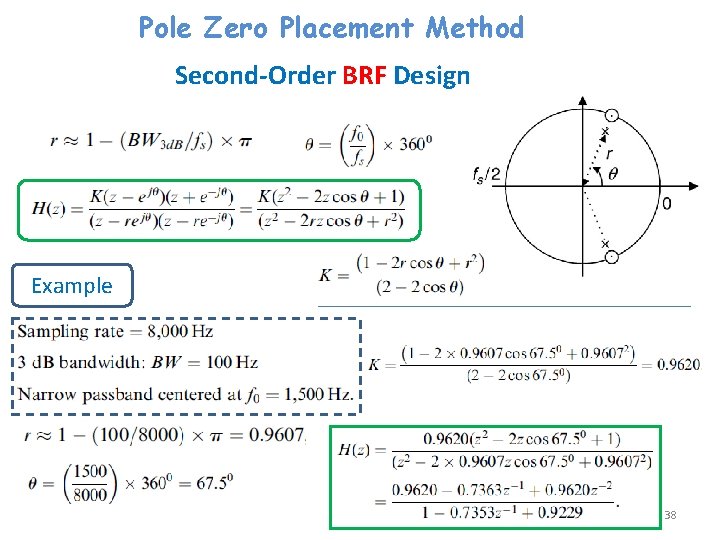
Pole Zero Placement Method Second-Order BRF Design Example 38

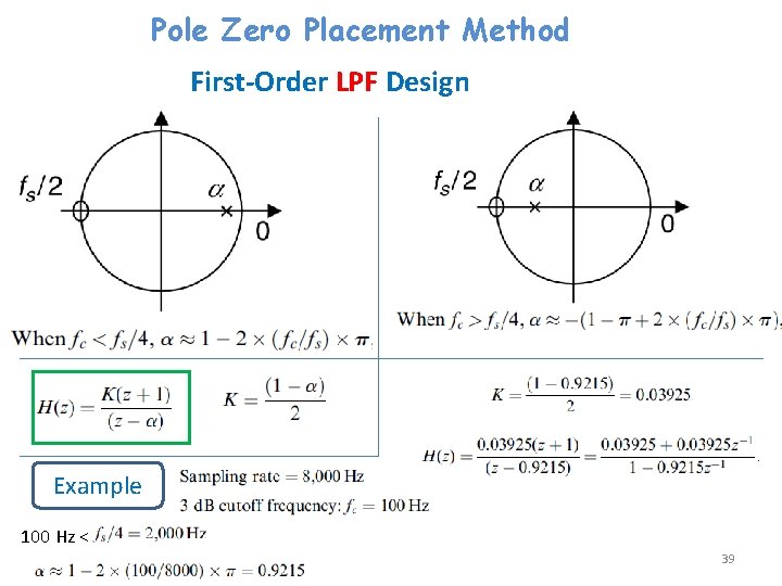
Pole Zero Placement Method First-Order LPF Design Example 100 Hz < 39

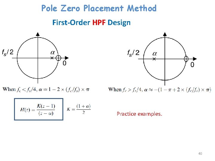
Pole Zero Placement Method First-Order HPF Design Practice examples. 40

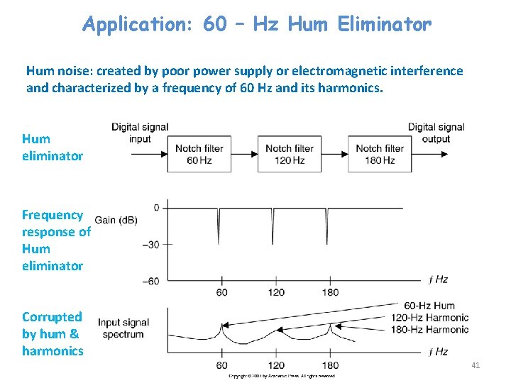
Application: 60 – Hz Hum Eliminator Hum noise: created by poor power supply or electromagnetic interference and characterized by a frequency of 60 Hz and its harmonics. Hum eliminator Frequency response of Hum eliminator Corrupted by hum & harmonics 41

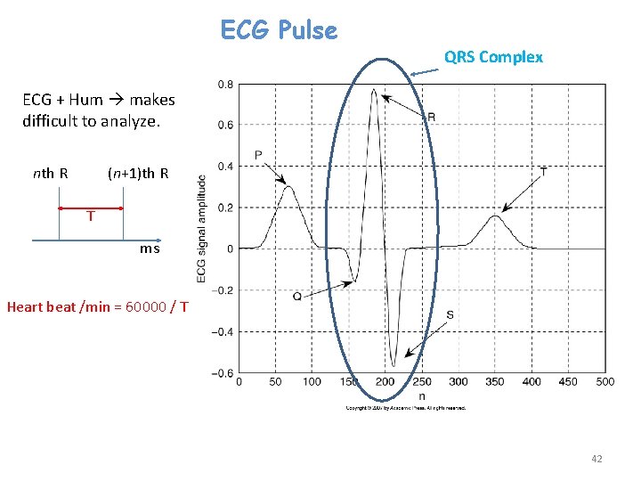
ECG Pulse QRS Complex ECG + Hum makes difficult to analyze. nth R (n+1)th R T ms Heart beat /min = 60000 / T 42

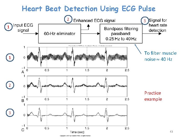
Heart Beat Detection Using ECG Pulse 2 3 1 1 To filter muscle noise 40 Hz 2 Practice example 3 43