DSPCIS PartIII Optimal Adaptive Filters Chapter10 Kalman Filters

DSP-CIS Part-III : Optimal & Adaptive Filters Chapter-10 : Kalman Filters Marc Moonen Dept. E. E. /ESAT-STADIUS, KU Leuven marc. moonen@kuleuven. be www. esat. kuleuven. be/stadius/

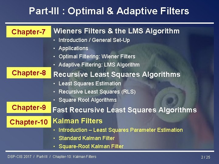
Part-III : Optimal & Adaptive Filters Chapter-7 Wieners Filters & the LMS Algorithm • • Introduction / General Set-Up Applications Optimal Filtering: Wiener Filters Adaptive Filtering: LMS Algorithm Chapter-8 – Recursive Least Squares Algorithms • Least Squares Estimation • Recursive Least Squares (RLS) • Square Root Algorithms Chapter-9 Fast Recursive Least Squares Algorithms Chapter-10 Kalman Filters • Introduction – Least Squares Parameter Estimation • Standard Kalman Filter • Square-Root Kalman Filter DSP-CIS 2017 / Part-III / Chapter-10: Kalman Filters 2 / 25

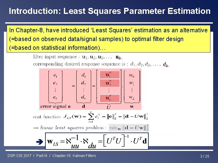
Introduction: Least Squares Parameter Estimation In Chapter-8, have introduced ‘Least Squares’ estimation as an alternative (=based on observed data/signal samples) to optimal filter design (=based on statistical information)… DSP-CIS 2017 / Part-III / Chapter-10: Kalman Filters 3 / 25

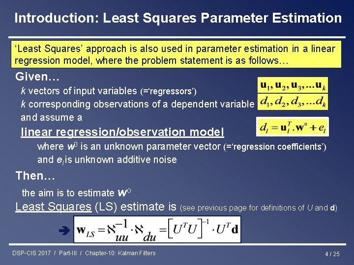
Introduction: Least Squares Parameter Estimation ‘Least Squares’ approach is also used in parameter estimation in a linear regression model, where the problem statement is as follows… Given… k vectors of input variables (=‘regressors’) k corresponding observations of a dependent variable and assume a linear regression/observation model where w 0 is an unknown parameter vector (=‘regression coefficients’) and el is unknown additive noise Then… the aim is to estimate wo Least Squares (LS) estimate is (see previous page for definitions of U and d) DSP-CIS 2017 / Part-III / Chapter-10: Kalman Filters 4 / 25

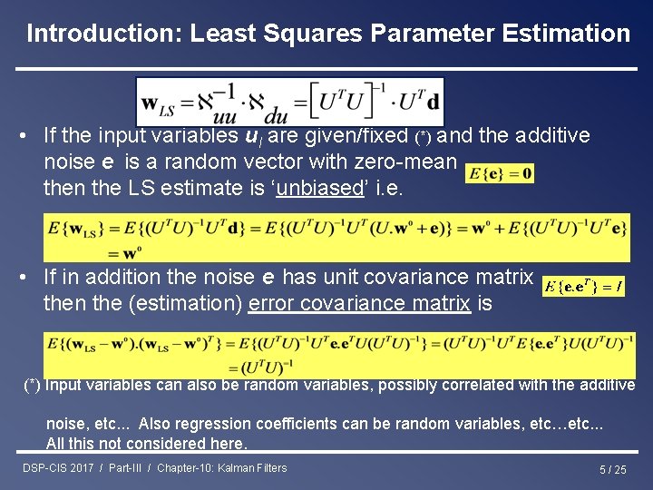
Introduction: Least Squares Parameter Estimation • If the input variables ul are given/fixed (*) and the additive noise e is a random vector with zero-mean the LS estimate is ‘unbiased’ i. e. • If in addition the noise e has unit covariance matrix then the (estimation) error covariance matrix is (*) Input variables can also be random variables, possibly correlated with the additive noise, etc. . . Also regression coefficients can be random variables, etc…etc. . . All this not considered here. DSP-CIS 2017 / Part-III / Chapter-10: Kalman Filters 5 / 25

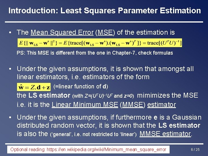
Introduction: Least Squares Parameter Estimation • The Mean Squared Error (MSE) of the estimation is PS: This MSE is different from the one in Chapter-7, check formulas • Under the given assumptions, it is shown that amongst all linear estimators, i. e. estimators of the form (=linear function of d) the LS estimator (with Z=(UTU)-1 UT and z=0) mimimizes the MSE i. e. it is the Linear Minimum MSE (MMSE) estimator • Under the given assumptions, if furthermore e is a Gaussian distributed random vector, it is shown that the LS estimator is also the (‘general’, i. e. not restricted to ‘linear’) MMSE estimator. DSP-CIS 2017 reading: / Part-III https: //en. wikipedia. org/wiki/Minimum_mean_square_error / Chapter-10: Kalman Filters Optional 6 / 25

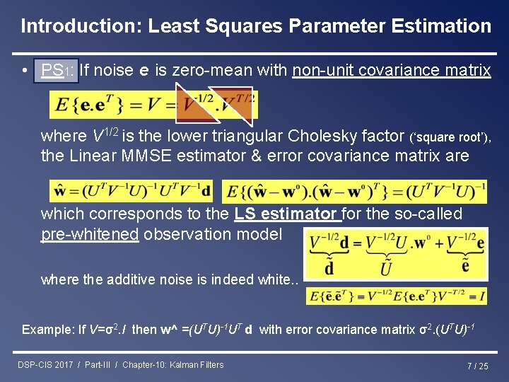
Introduction: Least Squares Parameter Estimation • PS 1: If noise e is zero-mean with non-unit covariance matrix where V 1/2 is the lower triangular Cholesky factor (‘square root’), the Linear MMSE estimator & error covariance matrix are which corresponds to the LS estimator for the so-called pre-whitened observation model where the additive noise is indeed white. . Example: If V=σ2. I then w^ =(UTU)-1 UT d with error covariance matrix σ2. (UTU)-1 DSP-CIS 2017 / Part-III / Chapter-10: Kalman Filters 7 / 25

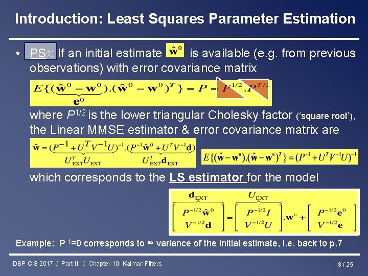
Introduction: Least Squares Parameter Estimation • PS 2: If an initial estimate is available (e. g. from previous observations) with error covariance matrix where P 1/2 is the lower triangular Cholesky factor (‘square root’), the Linear MMSE estimator & error covariance matrix are which corresponds to the LS estimator for the model Example: P-1=0 corresponds to ∞ variance of the initial estimate, i. e. back to p. 7 DSP-CIS 2017 / Part-III / Chapter-10: Kalman Filters 8 / 25

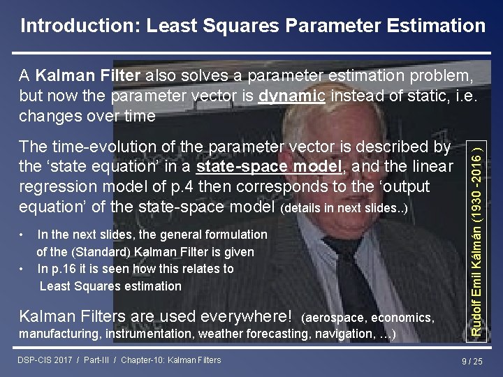
Introduction: Least Squares Parameter Estimation The time-evolution of the parameter vector is described by the ‘state equation’ in a state-space model, and the linear regression model of p. 4 then corresponds to the ‘output equation’ of the state-space model (details in next slides. . ) • • In the next slides, the general formulation of the (Standard) Kalman Filter is given In p. 16 it is seen how this relates to Least Squares estimation Kalman Filters are used everywhere! (aerospace, economics, manufacturing, instrumentation, weather forecasting, navigation, …) DSP-CIS 2017 / Part-III / Chapter-10: Kalman Filters Rudolf Emil Kálmán (1930 -2016 ) A Kalman Filter also solves a parameter estimation problem, but now the parameter vector is dynamic instead of static, i. e. changes over time 9 / 25

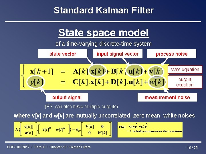
Standard Kalman Filter State space model of a time-varying discrete-time system state vector input signal vector process noise state equation output signal measurement noise (PS: can also have multiple outputs) where v[k] and w[k] are mutually uncorrelated, zero mean, white noises DSP-CIS 2017 / Part-III / Chapter-10: Kalman Filters 10 / 25

Standard Kalman Filter • Example: IIR filter u[k] + + -a 1 State space model is + -a 2 x bo y[k] + -a 3 x -a 4 x x x 1[k] x 2[k] x 3[k] x 4[k] b 1 b 2 b 3 b 4 x x + + x (no process/measurement noise here) DSP-CIS 2017 / Part-III / Chapter-10: Kalman Filters 11 / 25

Standard Kalman Filter State estimation problem state vector Given… A[k], B[k], C[k], D[k], V[k], W[k], k=0, 1, 2, . . . and input/output observations u[k], y[k], k=0, 1, 2, . . . Then… estimate the internal states x[k], k=0, 1, 2, . . . DSP-CIS 2017 / Part-III / Chapter-10: Kalman Filters 12 / 25

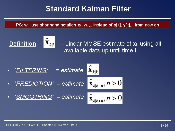
Standard Kalman Filter PS: will use shorthand notation xk, yk , . . instead of x[k], y[k], . . from now on Definition: • `FILTERING’ = Linear MMSE-estimate of xk using all available data up until time l = estimate • `PREDICTION’ = estimate • `SMOOTHING’ = estimate DSP-CIS 2017 / Part-III / Chapter-10: Kalman Filters 13 / 25

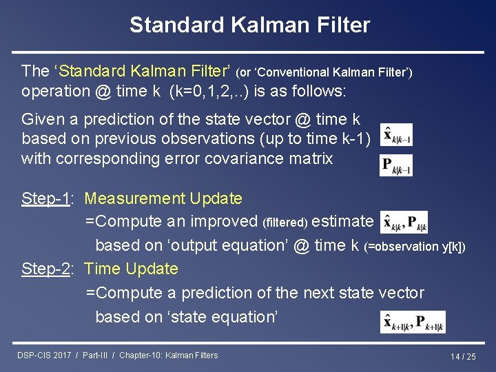
Standard Kalman Filter The ‘Standard Kalman Filter’ (or ‘Conventional Kalman Filter’) operation @ time k (k=0, 1, 2, . . ) is as follows: Given a prediction of the state vector @ time k based on previous observations (up to time k-1) with corresponding error covariance matrix Step-1: Measurement Update =Compute an improved (filtered) estimate based on ‘output equation’ @ time k (=observation y[k]) Step-2: Time Update =Compute a prediction of the next state vector based on ‘state equation’ DSP-CIS 2017 / Part-III / Chapter-10: Kalman Filters 14 / 25

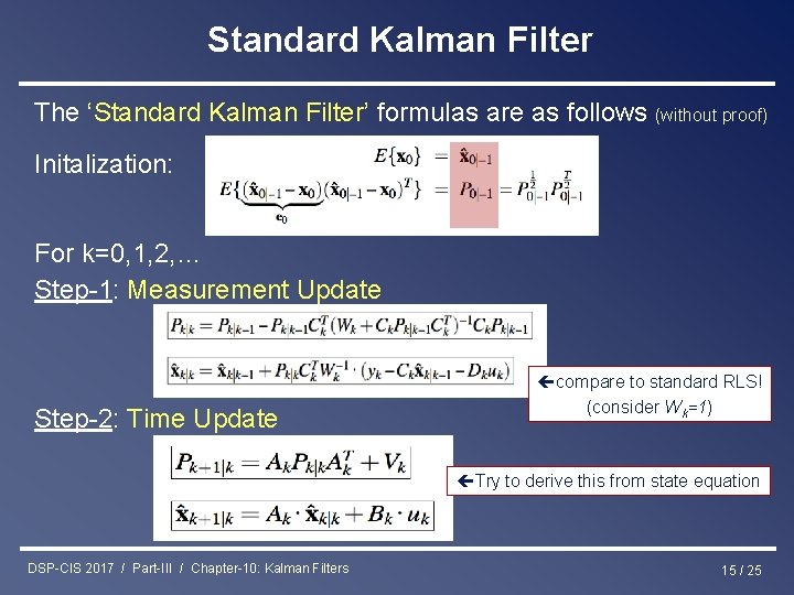
Standard Kalman Filter The ‘Standard Kalman Filter’ formulas are as follows (without proof) Initalization: For k=0, 1, 2, … Step-1: Measurement Update Step-2: Time Update compare to standard RLS! (consider Wk=1) Try to derive this from state equation DSP-CIS 2017 / Part-III / Chapter-10: Kalman Filters 15 / 25

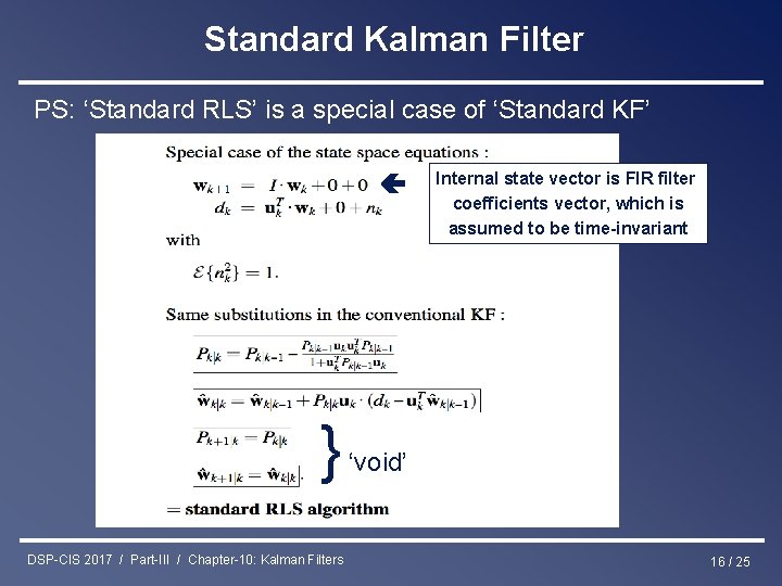
Standard Kalman Filter PS: ‘Standard RLS’ is a special case of ‘Standard KF’ } DSP-CIS 2017 / Part-III / Chapter-10: Kalman Filters Internal state vector is FIR filter coefficients vector, which is assumed to be time-invariant ‘void’ 16 / 25

Standard Kalman Filter PS: ‘Standard RLS’ is a special case of ‘Standard KF’ Standard RLS is not numerically stable (see Chapter-8), hence (similarly) the Standard KF is not numerically stable (i. e. finite precision implementation diverges from infinite precision implementation) Will therefore again derive an alternative Square-Root Algorithm which can be shown to be numerically stable (i. e. distance between finite precision implementation and infinite precision implementation is bounded) DSP-CIS 2017 / Part-III / Chapter-10: Kalman Filters 17 / 25

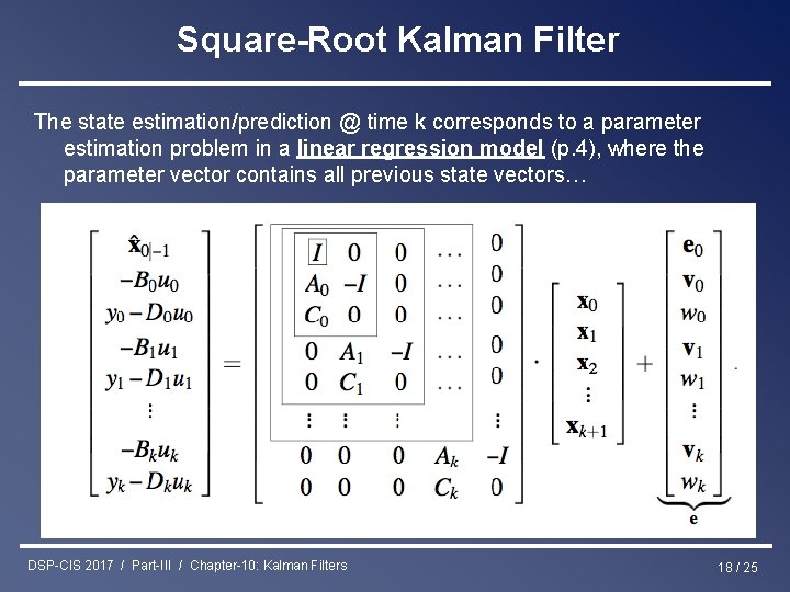
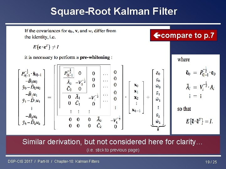
Square-Root Kalman Filter The state estimation/prediction @ time k corresponds to a parameter estimation problem in a linear regression model (p. 4), where the parameter vector contains all previous state vectors… DSP-CIS 2017 / Part-III / Chapter-10: Kalman Filters 18 / 25

Square-Root Kalman Filter compare to p. 7 Similar derivation, but not considered here for clarity… (i. e. stick to previous page) DSP-CIS 2017 / Part-III / Chapter-10: Kalman Filters 19 / 25

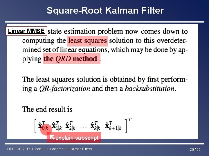
Square-Root Kalman Filter Linear MMSE explain subscript DSP-CIS 2017 / Part-III / Chapter-10: Kalman Filters 20 / 25

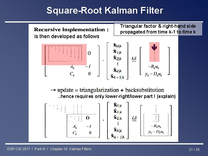
Square-Root Kalman Filter is then developed as follows Triangular factor & right-hand side propagated from time k-1 to time k . . hence requires only lower-right/lower part ! (explain) DSP-CIS 2017 / Part-III / Chapter-10: Kalman Filters 21 / 25

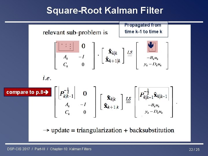
Square-Root Kalman Filter Propagated from time k-1 to time k compare to p. 8 DSP-CIS 2017 / Part-III / Chapter-10: Kalman Filters 22 / 25

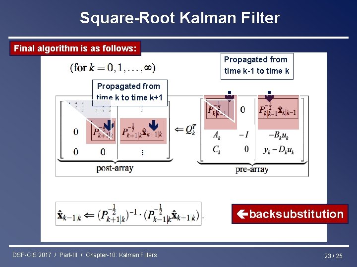
Square-Root Kalman Filter Final algorithm is as follows: Propagated from time k to time k+1 Propagated from time k-1 to time k backsubstitution DSP-CIS 2017 / Part-III / Chapter-10: Kalman Filters 23 / 25

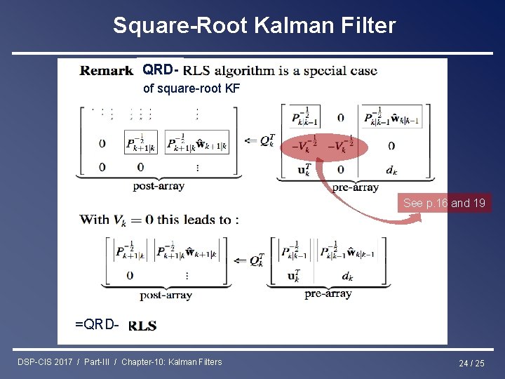
Square-Root Kalman Filter QRDof square-root KF See p. 16 and 19 =QRDDSP-CIS 2017 / Part-III / Chapter-10: Kalman Filters 24 / 25

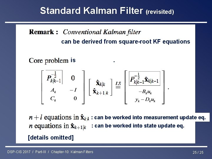
Standard Kalman Filter (revisited) can be derived from square-root KF equations is . : can be worked into measurement update eq. : can be worked into state update eq. [details omitted] DSP-CIS 2017 / Part-III / Chapter-10: Kalman Filters 25 / 25