FIR Filter Design Using Windows 1 The FIR

FIR Filter Design Using Windows 1

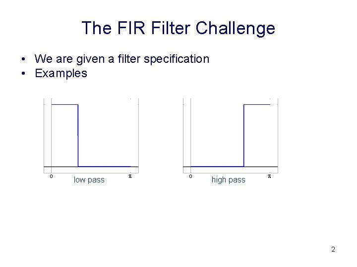
The FIR Filter Challenge • We are given a filter specification • Examples 0 low pass p 0 high pass p 2

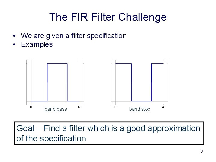
The FIR Filter Challenge • We are given a filter specification • Examples 0 band pass p 0 band stop p Goal – Find a filter which is a good approximation of the specification 3

Outline • • Goals Impulse Response truncation Using Windows Practical Filter Design 4

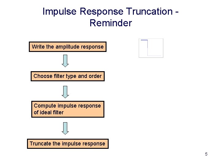
Impulse Response Truncation Reminder Write the amplitude response Choose filter type and order Compute impulse response of ideal filter Truncate the impulse response 5

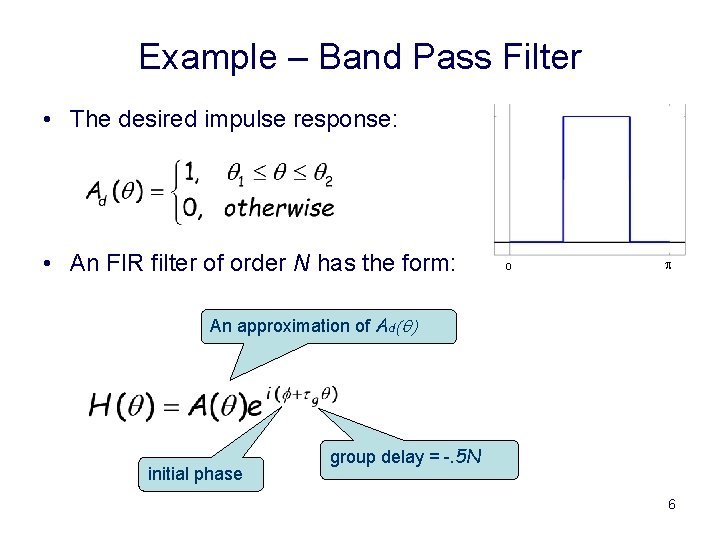
Example – Band Pass Filter • The desired impulse response: • An FIR filter of order N has the form: 0 p An approximation of Ad(q) initial phase group delay = -. 5 N 6

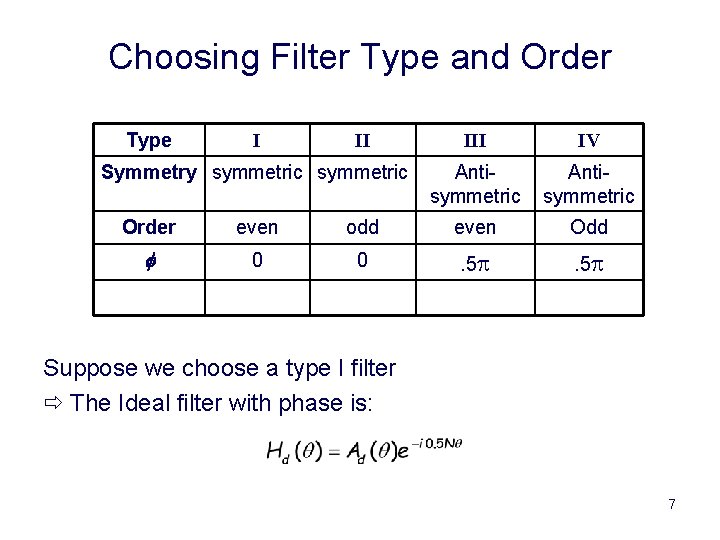
Choosing Filter Type and Order Type I II Symmetry symmetric III IV Antisymmetric Order even odd even Odd f 0 0 . 5 p Suppose we choose a type I filter ð The Ideal filter with phase is: 7

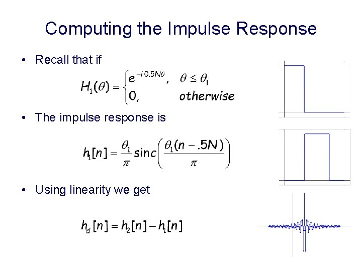
Computing the Impulse Response • Recall that if • The impulse response is • Using linearity we get 8

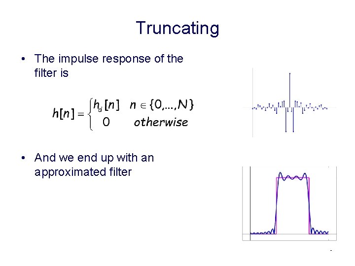
Truncating • The impulse response of the filter is • And we end up with an approximated filter 9

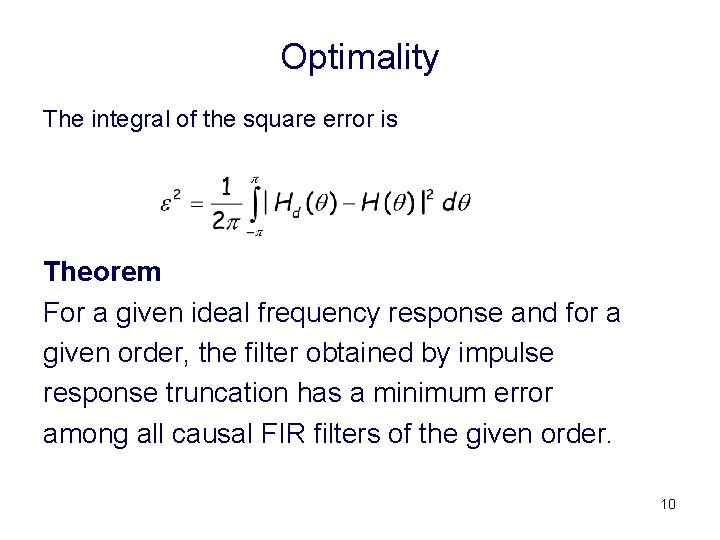
Optimality The integral of the square error is Theorem For a given ideal frequency response and for a given order, the filter obtained by impulse response truncation has a minimum error among all causal FIR filters of the given order. 10

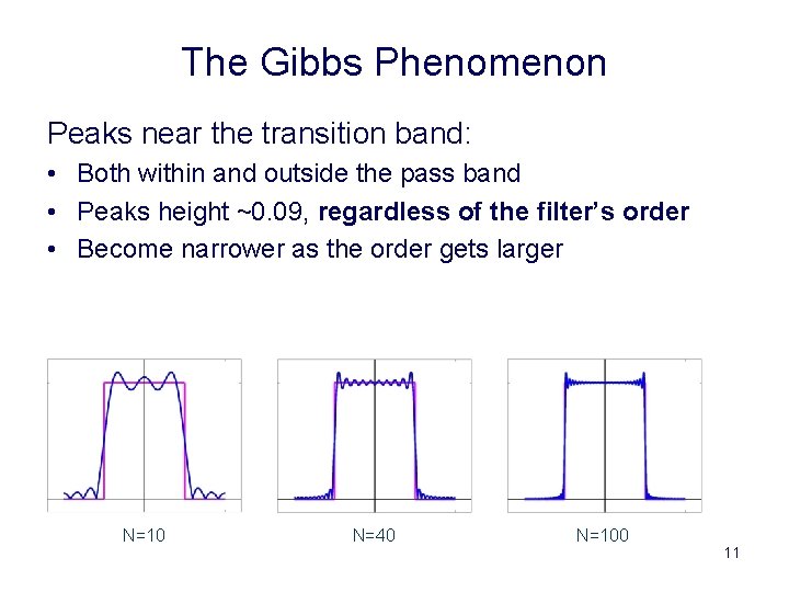
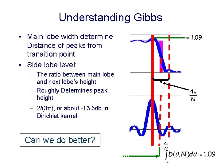
The Gibbs Phenomenon Peaks near the transition band: • Both within and outside the pass band • Peaks height ~0. 09, regardless of the filter’s order • Become narrower as the order gets larger N=10 N=40 N=100 11

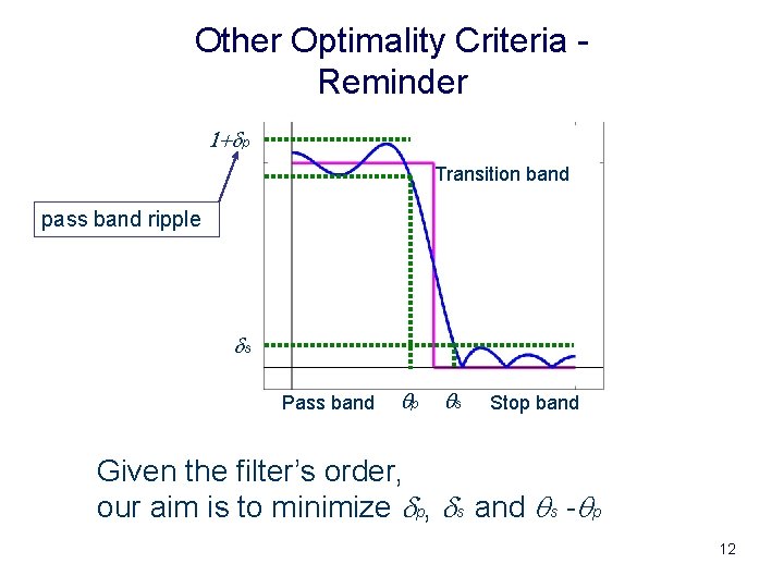
Other Optimality Criteria Reminder 1+dp Transition band pass band ripple ds Pass band qp qs Stop band Given the filter’s order, our aim is to minimize dp, ds and qs -qp 12

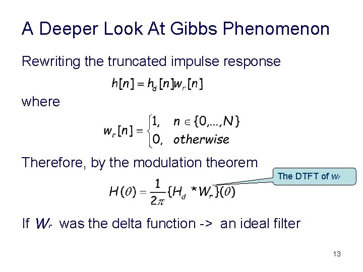
A Deeper Look At Gibbs Phenomenon Rewriting the truncated impulse response where Therefore, by the modulation theorem The DTFT of wr If Wr was the delta function -> an ideal filter 13

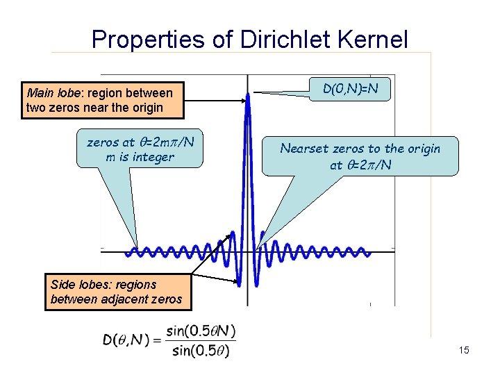
The DTFT of a Rectangular Window Suppose wr is a window with length N. The fourier transform of wr is: The function Is called the Dirichlet kernel 14

Properties of Dirichlet Kernel Main lobe: region between two zeros near the origin zeros at q=2 mp/N m is integer D(0, N)=N Nearset zeros to the origin at q=2 p/N Side lobes: regions between adjacent zeros 15

Understanding Gibbs • Main lobe width determine Distance of peaks from transition point • Side lobe level: – The ratio between main lobe and next lobe’s height – Roughly Determines peak height – 2/(3 p), or about -13. 5 db in Dirichlet kernel Can we do better? 16

Outline • • Goals Impulse Response truncation Using Windows Practical Filter Design 17

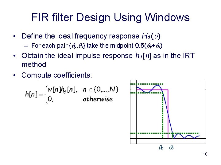
FIR filter Design Using Windows • Define the ideal frequency response Hd (q) – For each pair {qp, qs} take the midpoint 0. 5(qp+qs) • Obtain the ideal impulse response hd [n] as in the IRT method • Compute coefficients: qp qs 18

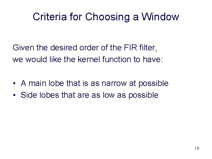
Criteria for Choosing a Window Given the desired order of the FIR filter, we would like the kernel function to have: • A main lobe that is as narrow at possible • Side lobes that are as low as possible 19

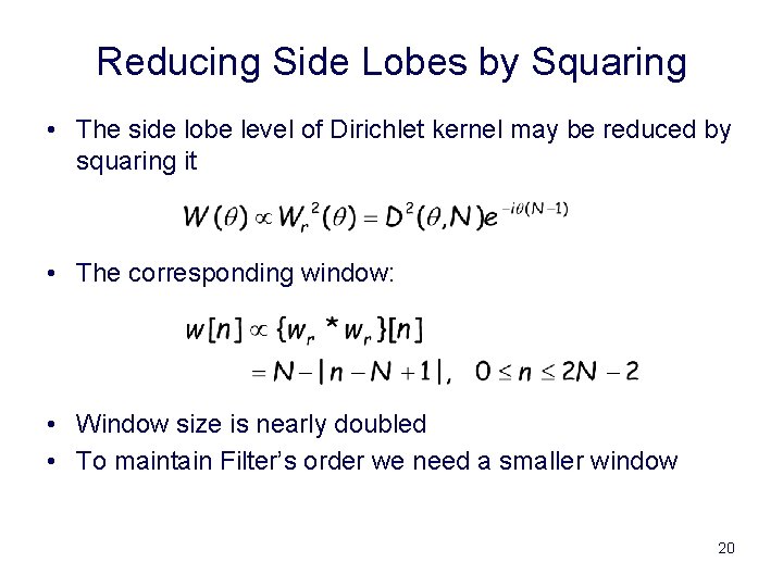
Reducing Side Lobes by Squaring • The side lobe level of Dirichlet kernel may be reduced by squaring it • The corresponding window: • Window size is nearly doubled • To maintain Filter’s order we need a smaller window 20

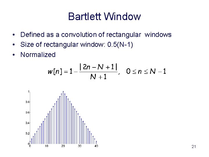
Bartlett Window • Defined as a convolution of rectangular windows • Size of rectangular window: 0. 5(N-1) • Normalized 21

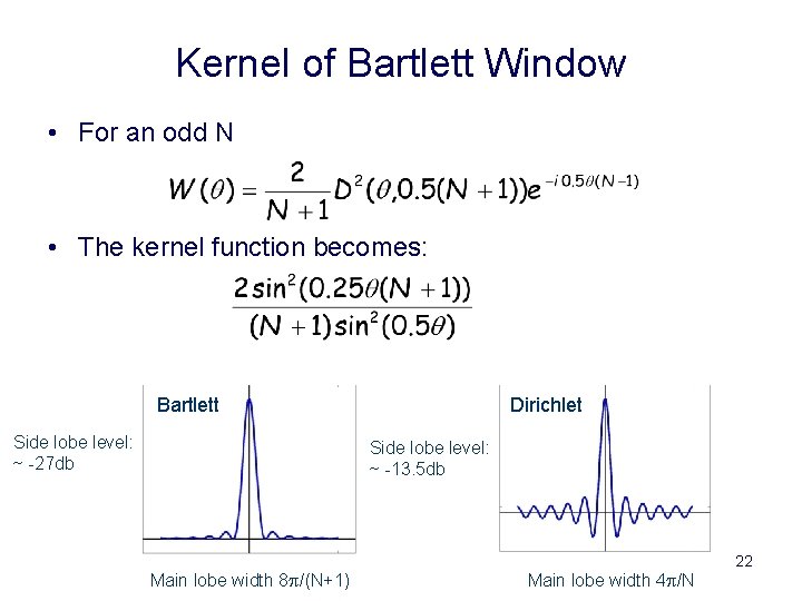
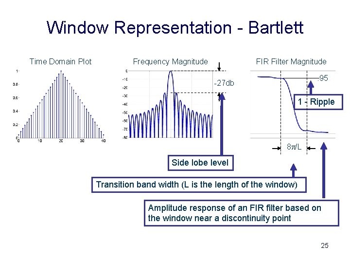
Kernel of Bartlett Window • For an odd N • The kernel function becomes: Bartlett Side lobe level: ~ -27 db Dirichlet Side lobe level: ~ -13. 5 db Main lobe width 8 p/(N+1) Main lobe width 4 p/N 22

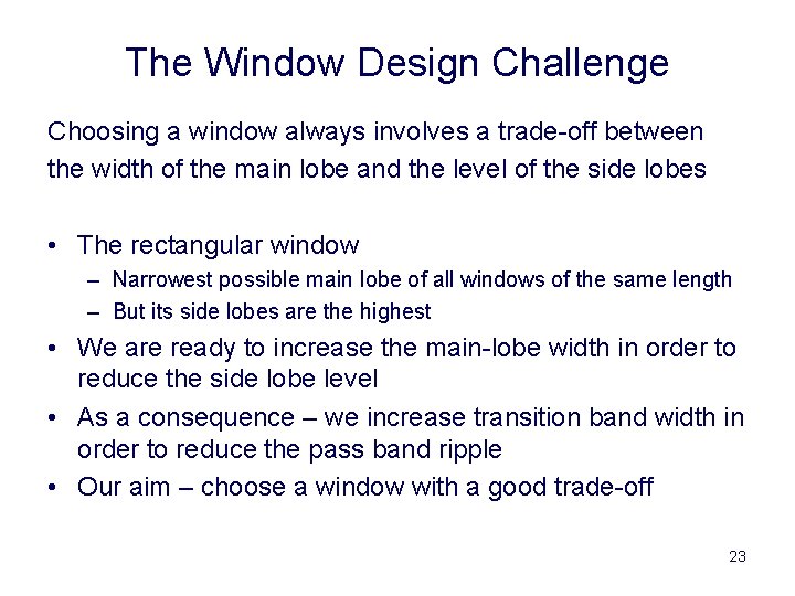
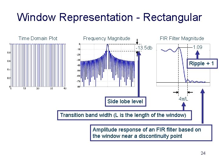
The Window Design Challenge Choosing a window always involves a trade-off between the width of the main lobe and the level of the side lobes • The rectangular window – Narrowest possible main lobe of all windows of the same length – But its side lobes are the highest • We are ready to increase the main-lobe width in order to reduce the side lobe level • As a consequence – we increase transition band width in order to reduce the pass band ripple • Our aim – choose a window with a good trade-off 23

Window Representation - Rectangular Time Domain Plot Frequency Magnitude FIR Filter Magnitude 1. 09 -13. 5 db Ripple + 1 Side lobe level 4 p/L Transition band width (L is the length of the window) Amplitude response of an FIR filter based on the window near a discontinuity point 24

Window Representation - Bartlett Time Domain Plot Frequency Magnitude FIR Filter Magnitude. 95 -27 db 1 - Ripple 8 p/L Side lobe level Transition band width (L is the length of the window) Amplitude response of an FIR filter based on the window near a discontinuity point 25

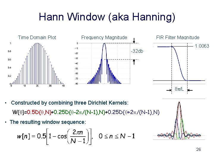
Hann Window (aka Hanning) Time Domain Plot Frequency Magnitude FIR Filter Magnitude 1. 0063. 95 -32 db 8 p/L • Constructed by combining three Dirichlet Kernels: W(q)=0. 5 D(q, N)+0. 25 D(q-2 p/(N-1), N)+0. 25 D(q+2 p/(N-1), N) • The resulting window sequence: 26

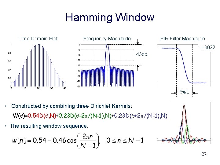
Hamming Window Time Domain Plot Frequency Magnitude FIR Filter Magnitude 1. 0022. 95 -43 db 8 p/L • Constructed by combining three Dirichlet Kernels: W(q)=0. 54 D(q, N)+0. 23 D(q-2 p/(N-1), N)+0. 23 D(q+2 p/(N-1), N) • The resulting window sequence: 27

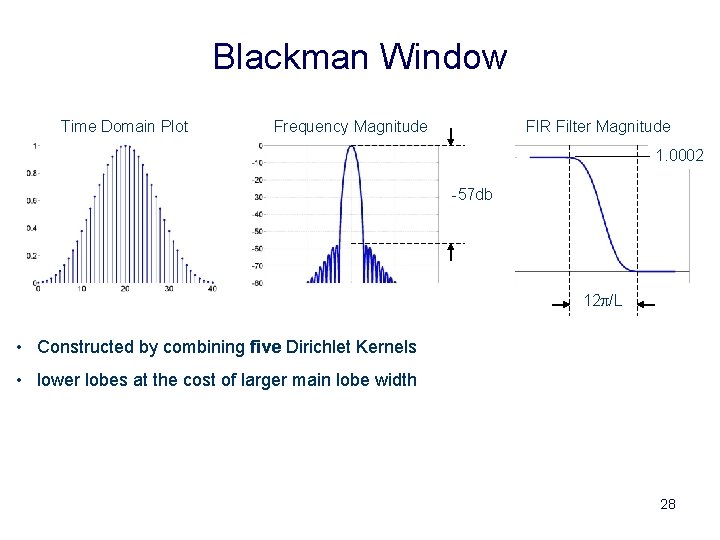
Blackman Window Time Domain Plot Frequency Magnitude FIR Filter Magnitude 1. 0002. 95 -57 db 12 p/L • Constructed by combining five Dirichlet Kernels • lower lobes at the cost of larger main lobe width 28

Optimal Windows • Previous windows were derived by intuition and educated guess • Modern windows are based on optimality criteria • Kaiser’s criterion – Minimize the width of the main lobe kernel – Constraints: • Window length should be fixed • Energy in the side lobes level do not exceed a percentage of total energy • Dolph criterion – Similar to Kaiser’s, except • Energy in side lobes do not exceed a given maximum value 29

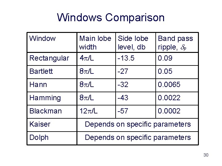
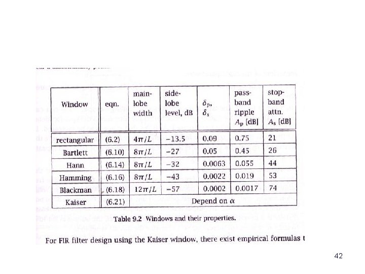
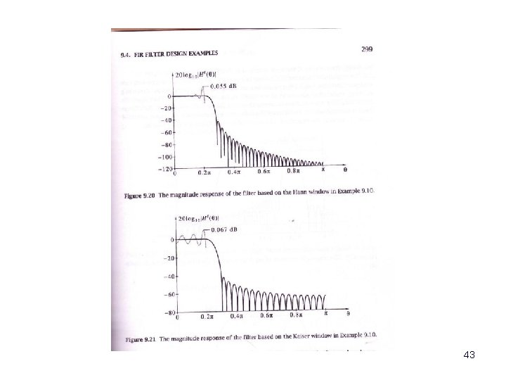
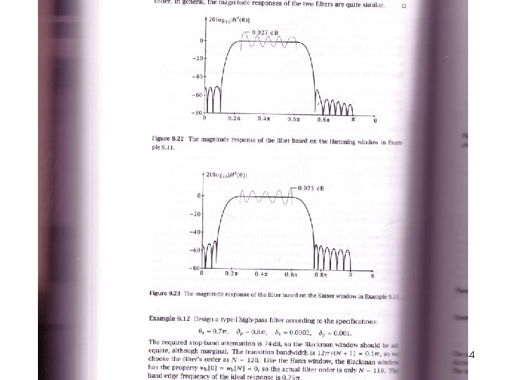
Windows Comparison Window Rectangular Main lobe Side lobe width level, db 4 p/L -13. 5 Band pass ripple, dp 0. 09 Bartlett 8 p/L -27 0. 05 Hann 8 p/L -32 0. 0065 Hamming 8 p/L -43 0. 0022 Blackman 12 p/L -57 0. 0002 Kaiser Depends on specific parameters Dolph Depends on specific parameters 30

Summary of Design by Windows • FIR design by impulse response truncation is optimal on the average • However, it is not optimal given constrained criteria • Windowing allows to tradeoff transition band width and pass band ripple • Specific window should be chosen according to desired constraints Recall that this is not the optimal method 31

Outline • • Goals Impulse Response truncation Using Windows Practical Filter Design 32

Designing a Filter We can use the function fir 1 theta=[-pi: 2*pi/1023: pi]; tf = fir 1(40, 0. 5, 'low', rectwin(41)); plot(theta, fftshift(abs(fft(tf, 1024)))); 33

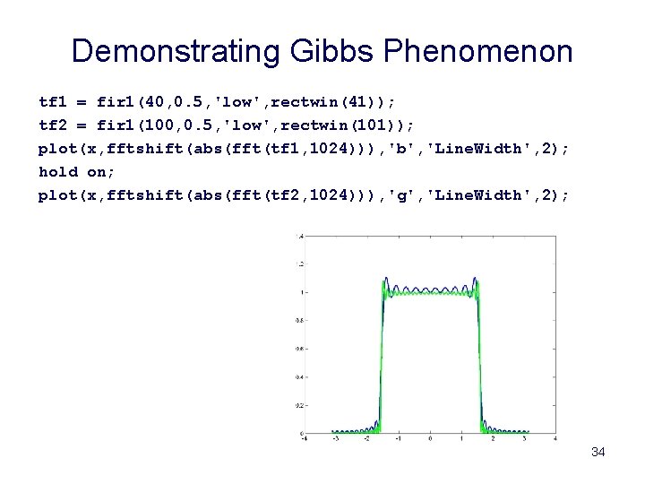
Demonstrating Gibbs Phenomenon tf 1 = fir 1(40, 0. 5, 'low', rectwin(41)); tf 2 = fir 1(100, 0. 5, 'low', rectwin(101)); plot(x, fftshift(abs(fft(tf 1, 1024))), 'b', 'Line. Width', 2); hold on; plot(x, fftshift(abs(fft(tf 2, 1024))), 'g', 'Line. Width', 2); 34

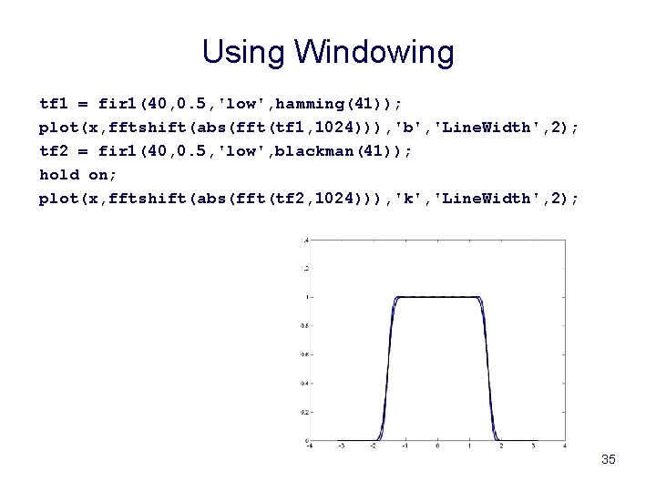
Using Windowing tf 1 = fir 1(40, 0. 5, 'low', hamming(41)); plot(x, fftshift(abs(fft(tf 1, 1024))), 'b', 'Line. Width', 2); tf 2 = fir 1(40, 0. 5, 'low', blackman(41)); hold on; plot(x, fftshift(abs(fft(tf 2, 1024))), 'k', 'Line. Width', 2); 35

Using Least Square Design lsf=firls(40, [0 0. 5001 1], [1 1 0 0]); plot(x, fftshift(abs(fft(lsf, 1024))), 'b', 'Line. Width', 2); hold on; lsf 2=firls(40, [0 0. 5 0. 6 1], [1 1 0 0]); plot(x, fftshift(abs(fft(lsf 2, 1024))), 'k', 'Line. Width', 2); 36

Usign Remez Exchange Re. F=remez(40, [0 0. 5 0. 6 1], [1 1 0 0]); plot(x, fftshift(abs(fft(Re. F, 1024))), 'k', 'Line. Width', 2); 37

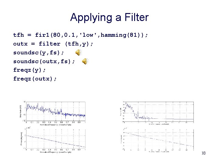
Applying a Filter tfh = fir 1(80, 0. 1, 'low', hamming(81)); outx = filter (tfh, y); soundsc(y, fs); soundsc(outx, fs); freqz(y); freqz(outx); 38

Beyond Low-pass lsf=firls(500, [0 0. 4001 0. 6001 0. 7001 1], … [0 0 5 5 10 10 0 0]); outx = filter(lsf, 1, y); plot(x, fftshift(abs(fft(lsf, 1024))), 'b', 'Line. Width', 2); soundsc(outx, fs); plot(outx, fftshift(abs(fft(lsf, 1024))), 'b', 'Line. Width', 2); 39

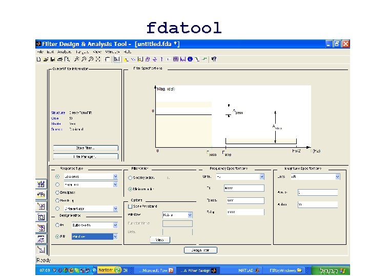
fdatool 40

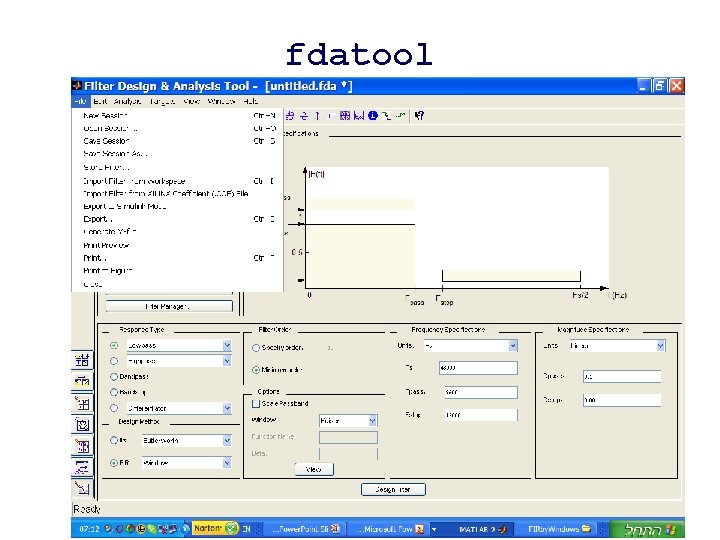
fdatool 41

42

43

44