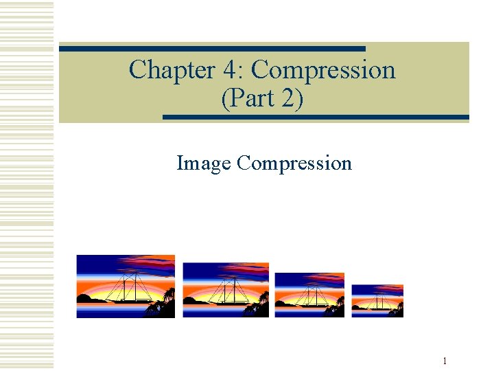
Chapter 4 Compression Part 2 Image Compression 1

Chapter 4: Compression (Part 2) Image Compression 1

Acknowledgement w Some figures and pictures are taken from: The Scientist and Engineer's Guide to Digital Signal Processing by Steven W. Smith 2

Lossy compression w Motivations: n n n Uncompressed images, video and audio data are huge, e. g. , in HDTV, bit rate easily exceeds 1 Gbps. Lossless methods (Huffman, Arithmetic, LZW) are inadequate for images and video because the spatial and/or temporal redundancy of pixel values are not exploited. Special characteristics of human perception (e. g. , more sensitive to low spatial frequencies) should be taken advantage of to achieve a higher compression ratio. 3

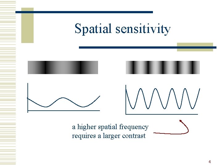
Spatial sensitivity a higher spatial frequency requires a larger contrast 4

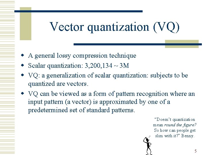
Vector quantization (VQ) w A general lossy compression technique w Scalar quantization: 3, 200, 134 ~ 3 M w VQ: a generalization of scalar quantization: subjects to be quantized are vectors. w VQ can be viewed as a form of pattern recognition where an input pattern (a vector) is approximated by one of a predetermined set of standard patterns. “Doesn’t quantization mean round the figure? So how can people get slim with it? ” Benny. 5

Vector quantization (Def’n) w A vector quantizer Q of dimension k and size N is a mapping from a vector in a k-dimensional Euclidean space into a finite set C containing N output or reproduction points, called code vectors. k Vector Q C N w C: the codebook (with N vectors). 6

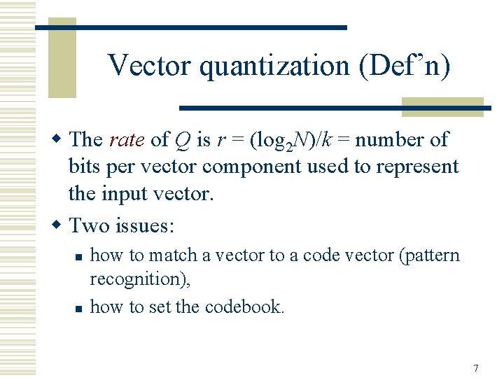
Vector quantization (Def’n) w The rate of Q is r = (log 2 N)/k = number of bits per vector component used to represent the input vector. w Two issues: n n how to match a vector to a code vector (pattern recognition), how to set the codebook. 7

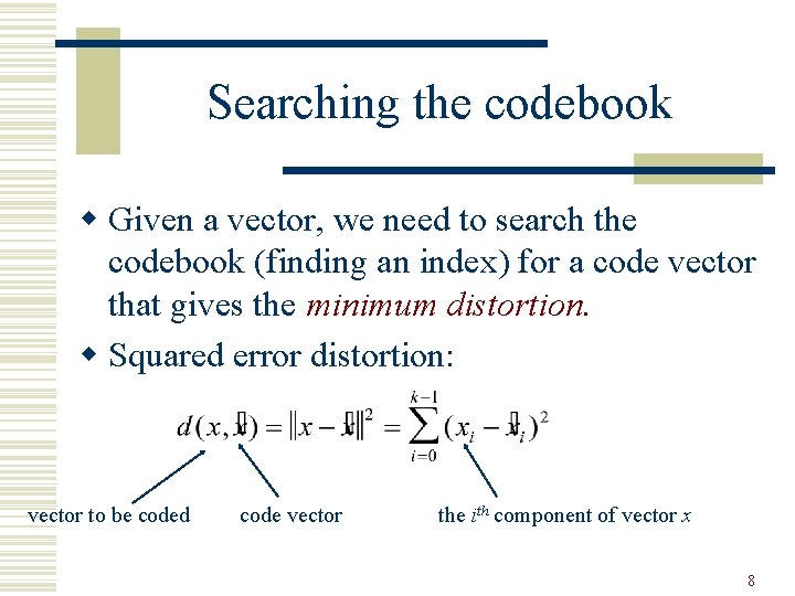
Searching the codebook w Given a vector, we need to search the codebook (finding an index) for a code vector that gives the minimum distortion. w Squared error distortion: vector to be coded code vector the ith component of vector x 8

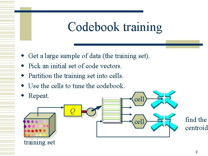
Codebook training w w w Get a large sample of data (the training set). Pick an initial set of code vectors. Partition the training set into cells. Use the cells to tune the codebook. Repeat. cell Q cell find the centroid training set 9

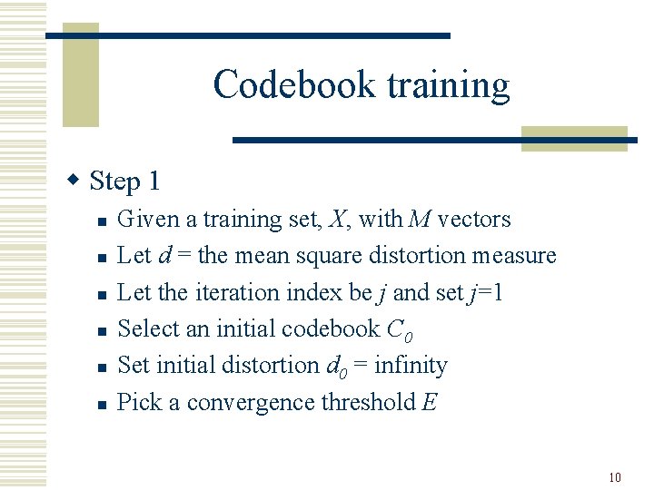
Codebook training w Step 1 n n n Given a training set, X, with M vectors Let d = the mean square distortion measure Let the iteration index be j and set j=1 Select an initial codebook C 0 Set initial distortion d 0 = infinity Pick a convergence threshold E 10

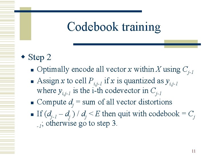
Codebook training w Step 2 n n Optimally encode all vector x within X using Cj-1 Assign x to cell Pi, j-1 if x is quantized as yi, j-1 where yi, j-1 is the i-th codevector in Cj-1 Compute dj = sum of all vector distortions If (dj-1 – dj ) / dj < E then quit with codebook = Cj -1; otherwise go to step 3. 11

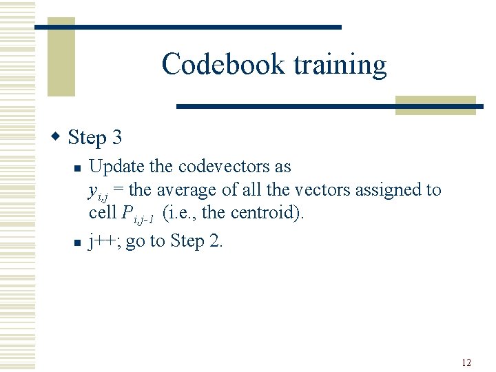
Codebook training w Step 3 n n Update the codevectors as yi, j = the average of all the vectors assigned to cell Pi, j-1 (i. e. , the centroid). j++; go to Step 2. 12

Codebook training (illustration) vector 1 [25, 10, 24] 2 [30, 30] 3 [11, 91, 11] 00 [25, 33, 40] 4 [28, 29] 01 [13, 53, 61] 5 [20, 81, 11] 6 [15, 42, 52] 10 [20, 88, 30] 7 [24, 11, 24] 11 [21, 10, 24] 8 [28, 29, 28] 9 [25, 12, 25] 10 [10, 89, 12] code set code vector codebook training vectors 13

Codebook training (illustration) vector 1 [25, 10, 24] 2 [30, 30] 3 [11, 91, 11] 00 [25, 33, 40] 4 [28, 29] 01 [13, 53, 61] 5 [20, 81, 11] 6 [15, 42, 52] 10 [20, 88, 30] 7 [24, 11, 24] 11 [21, 10, 24] 8 [28, 29, 28] 9 [25, 12, 25] 10 [10, 89, 12] training vectors code set code vector codebook d([25, 10, 24], [25, 33, 40]) = 785 d([25, 10, 24], [13, 53, 61]) = 3362 d([25, 10, 24], [20, 88, 30]) = 6145 d([25, 10, 24], [21, 10, 24]) = 16 14

Codebook training (illustration) vector 1 [25, 10, 24] 2 [30, 30] 3 [11, 91, 11] 00 [25, 33, 40] 4 [28, 29] 01 [13, 53, 61] 5 [20, 81, 11] 6 [15, 42, 52] 10 [20, 88, 30] 7 [24, 11, 24] 8 [28, 29, 28] 9 [25, 12, 25] 10 [10, 89, 12] training vectors code 11 set 1 code vector [21, 10, 24] codebook d([25, 10, 24], [25, 33, 40]) = 785 d([25, 10, 24], [13, 53, 61]) = 3362 d([25, 10, 24], [20, 88, 30]) = 6145 d([25, 10, 24], [21, 10, 24]) = 16 15

Codebook training (illustration) vector 1 [25, 10, 24] 2 [30, 30] 3 code set code vector [11, 91, 11] 00 2, 4, 8 [25, 33, 40] 4 [28, 29] 01 6 [13, 53, 61] 5 [20, 81, 11] 6 [15, 42, 52] 10 3, 5, 10 [20, 88, 30] 7 [24, 11, 24] 11 1, 7, 9 [21, 10, 24] 8 [28, 29, 28] 9 [25, 12, 25] 10 [10, 89, 12] codebook training vectors 16

Codebook training (illustration) vector 1 [25, 10, 24] 2 [30, 30] 3 code set code vector [11, 91, 11] 00 2, 4, 8 [25, 33, 40] 4 [28, 29] 01 6 [13, 53, 61] 5 [20, 81, 11] 6 [15, 42, 52] 10 3, 5, 10 [20, 88, 30] 7 [24, 11, 24] 11 1, 7, 9 [21, 10, 24] 8 [28, 29, 28] 9 [25, 12, 25] 10 [10, 89, 12] training vectors codebook [30, 30]+[28, 29]+[28, 29, 28] 3 = [28, 29] 17

Codebook training (illustration) vector 1 [25, 10, 24] 2 [30, 30] 3 code set code vector [11, 91, 11] 00 2, 4, 8 [28, 29] 4 [28, 29] 01 6 [15, 42, 52] 5 [20, 81, 11] 6 [15, 42, 52] 10 3, 5, 10 [13, 87, 11] 7 [24, 11, 24] 11 1, 7, 9 [24, 11, 24] 8 [28, 29, 28] 9 [25, 12, 25] 10 [10, 89, 12] codebook training vectors 18

Codebook training (illustration) vector code 1 [25, 10, 24] [24, 11, 24] 11 2 [30, 30] [28, 29] 00 3 [11, 91, 11] [13, 87, 11] 10 4 [28, 29] 00 5 [20, 81, 11] [13, 87, 11] 10 6 [15, 42, 52] 01 7 [24, 11, 24] 11 8 [28, 29, 28] [28, 29] 00 9 [25, 12, 25] [24, 11, 24] 11 10 [10, 89, 12] [13, 87, 11] 10 19

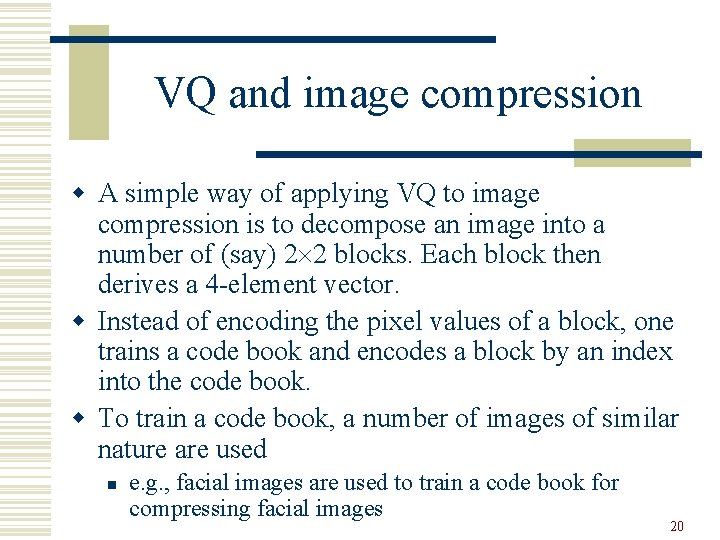
VQ and image compression w A simple way of applying VQ to image compression is to decompose an image into a number of (say) 2 2 blocks. Each block then derives a 4 -element vector. w Instead of encoding the pixel values of a block, one trains a code book and encodes a block by an index into the code book. w To train a code book, a number of images of similar nature are used n e. g. , facial images are used to train a code book for compressing facial images 20

[154, 147] [175, 182, 168, 154] [189, 168, 168] [217, 175, 196, 175] [175, 154, 175, 168] [203, 175, 168] … … 21

Image & video compression w JPEG: spatial redundancy removal in intraframe coding. w H. 261 and MPEG: both spatial and temporal redundancy removal in intra-frame and interframe coding. 22

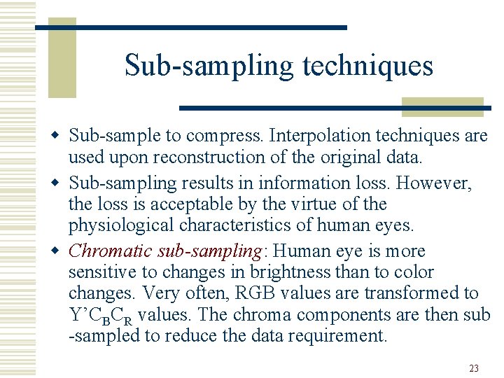
Sub-sampling techniques w Sub-sample to compress. Interpolation techniques are used upon reconstruction of the original data. w Sub-sampling results in information loss. However, the loss is acceptable by the virtue of the physiological characteristics of human eyes. w Chromatic sub-sampling: Human eye is more sensitive to changes in brightness than to color changes. Very often, RGB values are transformed to Y’CBCR values. The chroma components are then sub -sampled to reduce the data requirement. 23

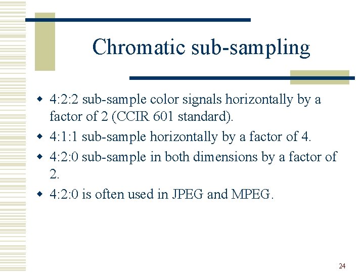
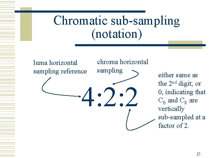
Chromatic sub-sampling w 4: 2: 2 sub-sample color signals horizontally by a factor of 2 (CCIR 601 standard). w 4: 1: 1 sub-sample horizontally by a factor of 4. w 4: 2: 0 sub-sample in both dimensions by a factor of 2. w 4: 2: 0 is often used in JPEG and MPEG. 24

Chromatic sub-sampling (notation) luma horizontal sampling reference chroma horizontal sampling 4: 2: 2 either same as the 2 nd digit; or 0, indicating that CB and CR are vertically sub-sampled at a factor of 2. 25

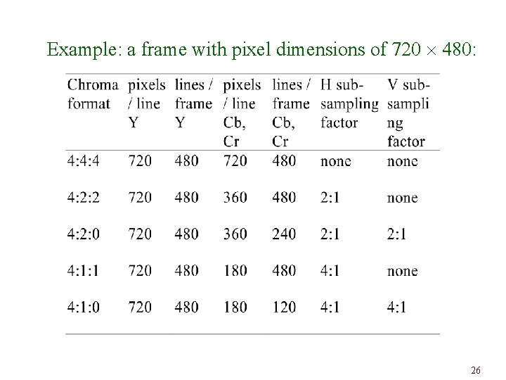
Example: a frame with pixel dimensions of 720 480: 26

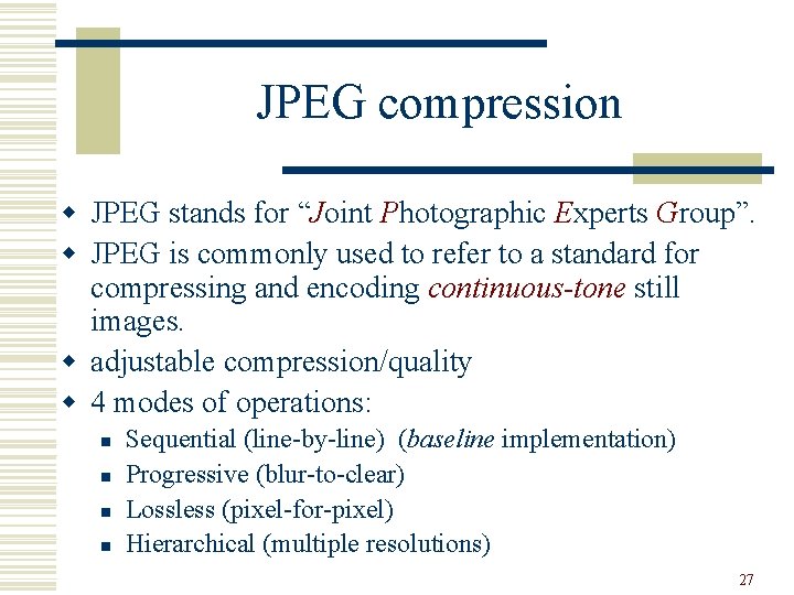
JPEG compression w JPEG stands for “Joint Photographic Experts Group”. w JPEG is commonly used to refer to a standard for compressing and encoding continuous-tone still images. w adjustable compression/quality w 4 modes of operations: n n Sequential (line-by-line) (baseline implementation) Progressive (blur-to-clear) Lossless (pixel-for-pixel) Hierarchical (multiple resolutions) 27

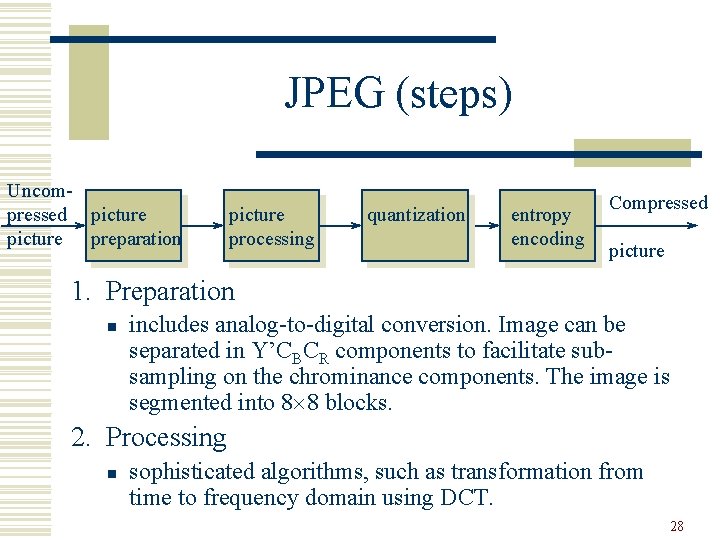
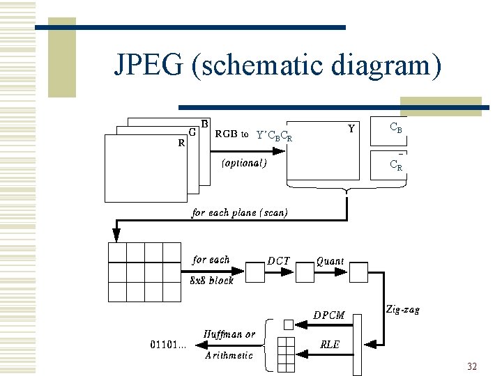
JPEG (steps) Uncompressed picture preparation picture processing quantization entropy encoding Compressed picture 1. Preparation n includes analog-to-digital conversion. Image can be separated in Y’CBCR components to facilitate subsampling on the chrominance components. The image is segmented into 8 8 blocks. 2. Processing n sophisticated algorithms, such as transformation from time to frequency domain using DCT. 28

1/4 1/2 1/2 29

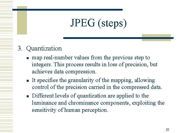
JPEG (steps) 3. Quantization n map real-number values from the previous step to integers. This process results in loss of precision, but achieves data compression. It specifies the granularity of the mapping, allowing control of the precision carried in the compressed data. Different levels of quantization are applied to the luminance and chrominance components, exploiting the sensitivity of human perception. 30

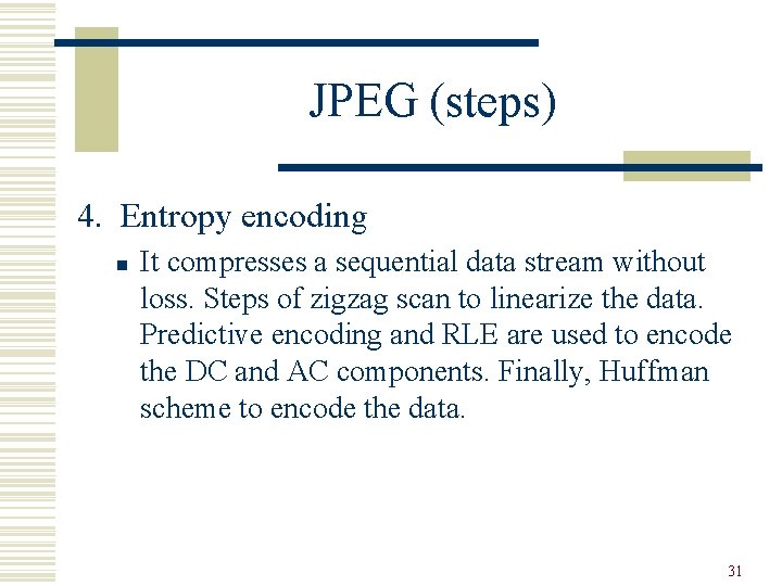
JPEG (steps) 4. Entropy encoding n It compresses a sequential data stream without loss. Steps of zigzag scan to linearize the data. Predictive encoding and RLE are used to encode the DC and AC components. Finally, Huffman scheme to encode the data. 31

JPEG (schematic diagram) Y’CBCR CB CR 32

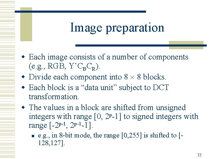
Image preparation w Each image consists of a number of components (e. g. , RGB, Y’CBCR). w Divide each component into 8 8 blocks. w Each block is a “data unit” subject to DCT transformation. w The values in a block are shifted from unsigned integers with range [0, 2 p-1] to signed integers with range [-2 p-1, 2 p-1 -1]. n e. g. , in 8 -bit mode, the range [0, 255] is shifted to [128, 127]. 33

34

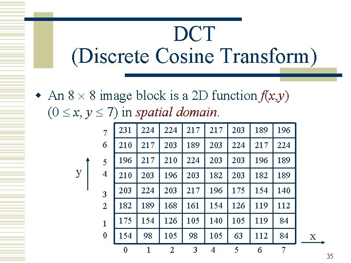
DCT (Discrete Cosine Transform) w An 8 8 image block is a 2 D function f(x, y) (0 x, y 7) in spatial domain. y 7 6 231 224 217 203 189 196 210 217 203 189 203 224 217 224 5 4 196 217 210 224 203 196 189 210 203 196 203 182 189 3 2 203 224 203 217 196 175 154 140 182 189 168 161 154 126 119 112 1 0 175 154 126 105 140 105 119 84 154 98 105 63 112 84 0 1 2 3 4 5 6 7 x 35

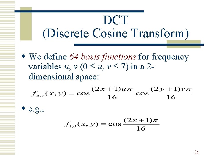
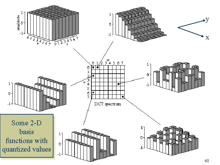
DCT (Discrete Cosine Transform) w We define 64 basis functions for frequency variables u, v (0 u, v 7) in a 2 dimensional space: w e. g. , 36

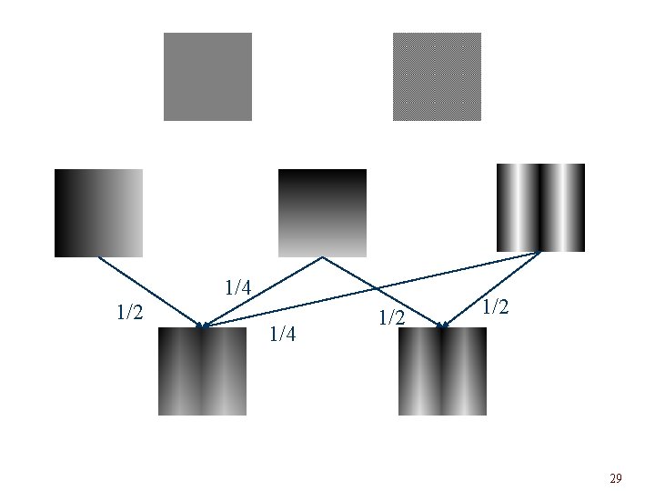
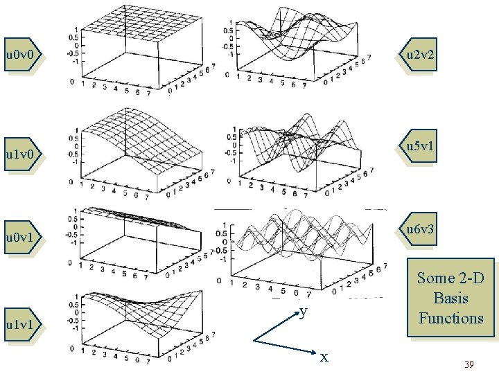
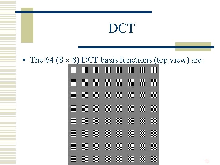
DCT (Discrete Cosine Transform) w These are wave functions of successively increasing frequencies. (Imagine them as undulating surfaces of increasingly frequent ups and downs. ) w Given a 2 D function (imagine it as a 2 D surface), one can decompose it into a linear combination of these wave functions. w So, DCT is a frequency (uv coordinates) representation of a spatial (xy coordinates) function. 37

A 1 -D example 38

u 0 v 0 u 2 v 2 u 5 v 1 u 1 v 0 u 6 v 3 u 0 v 1 u 1 v 1 Some 2 -D Basis Functions y x 39

y x Some 2 -D basis functions with quantized values 40

DCT w The 64 (8 8) DCT basis functions (top view) are: 41

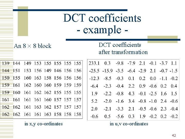
DCT coefficients - example An 8 8 block in x, y co-ordinates DCT coefficients after transformation in u, v co-ordinates 42

43

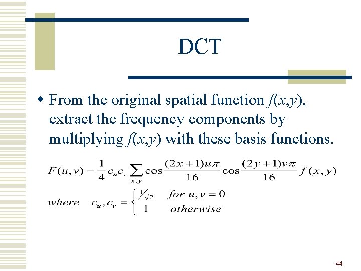
DCT w From the original spatial function f(x, y), extract the frequency components by multiplying f(x, y) with these basis functions. 44

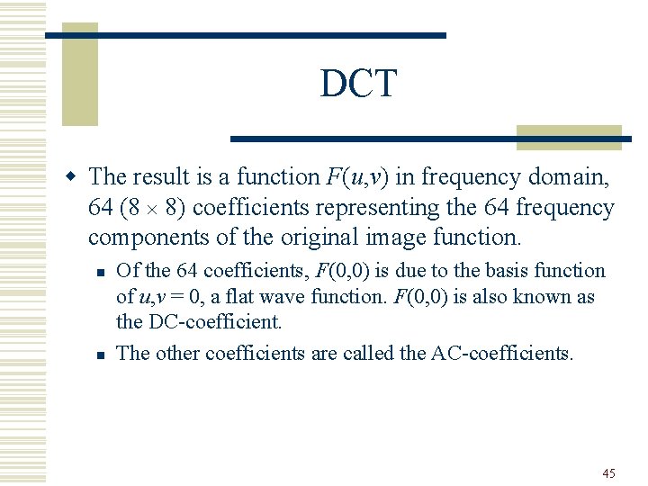
DCT w The result is a function F(u, v) in frequency domain, 64 (8 8) coefficients representing the 64 frequency components of the original image function. n n Of the 64 coefficients, F(0, 0) is due to the basis function of u, v = 0, a flat wave function. F(0, 0) is also known as the DC-coefficient. The other coefficients are called the AC-coefficients. 45

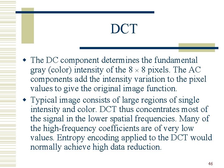
DCT w The DC component determines the fundamental gray (color) intensity of the 8 8 pixels. The AC components add the intensity variation to the pixel values to give the original image function. w Typical image consists of large regions of single intensity and color. DCT thus concentrates most of the signal in the lower spatial frequencies. Many of the high-frequency coefficients are of very low values. Entropy encoding applied to the DCT would normally achieve high data reduction. 46

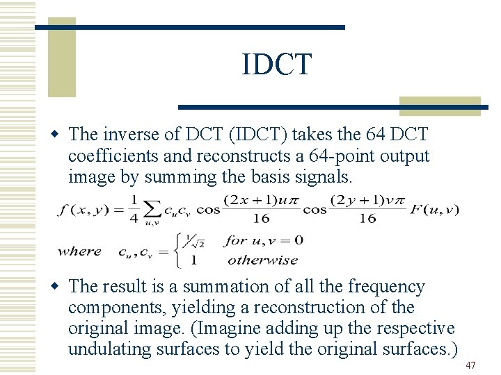
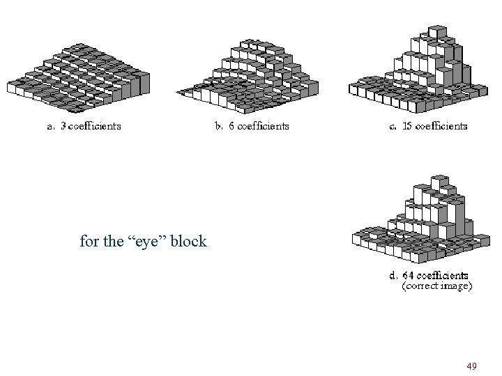
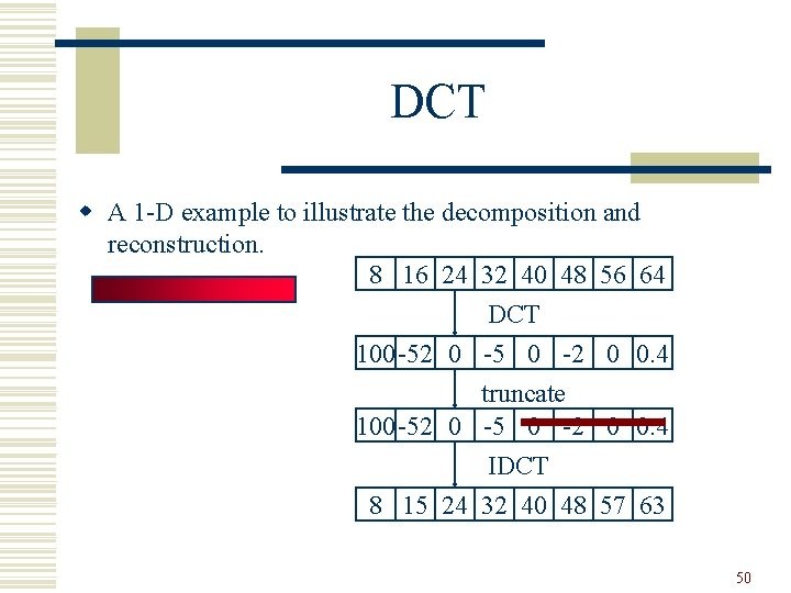
IDCT w The inverse of DCT (IDCT) takes the 64 DCT coefficients and reconstructs a 64 -point output image by summing the basis signals. w The result is a summation of all the frequency components, yielding a reconstruction of the original image. (Imagine adding up the respective undulating surfaces to yield the original surfaces. ) 47

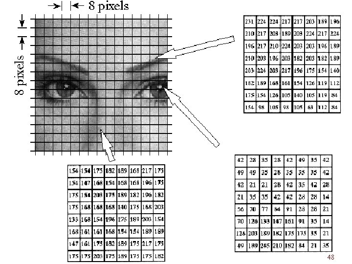
48

for the “eye” block 49

DCT w A 1 -D example to illustrate the decomposition and reconstruction. 8 16 24 32 40 48 56 64 DCT 100 -52 0 -5 0 -2 0 0. 4 truncate 100 -52 0 -5 0 -2 0 0. 4 IDCT 8 15 24 32 40 48 57 63 50

Quantization w The 64 DCT coefficients are real numbers (i. e. , not integers). These coefficients are quantized to throw away bits, and that is the main source of lossiness. 51

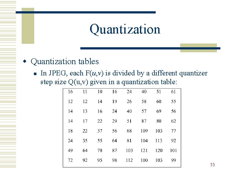
Quantization w Uniform quantization n n DCT coefficients can be divided by a constant N and the result is rounded. Equal treatment to all DCT coefficients. w Quantization tables n Each of the 64 coefficients can be adjusted separately. Specific frequencies can be given more importance than others according to the characteristics of the original image. 52

Quantization w Quantization tables n In JPEG, each F(u, v) is divided by a different quantizer step size Q(u, v) given in a quantization table: 53

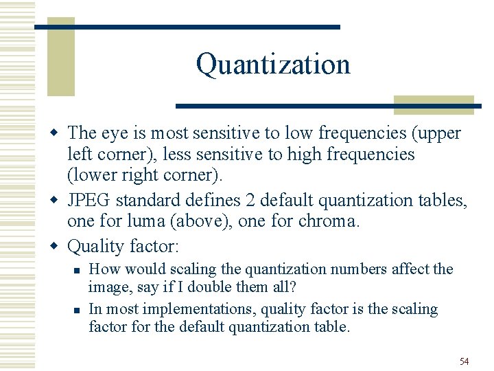
Quantization w The eye is most sensitive to low frequencies (upper left corner), less sensitive to high frequencies (lower right corner). w JPEG standard defines 2 default quantization tables, one for luma (above), one for chroma. w Quality factor: n n How would scaling the quantization numbers affect the image, say if I double them all? In most implementations, quality factor is the scaling factor for the default quantization table. 54

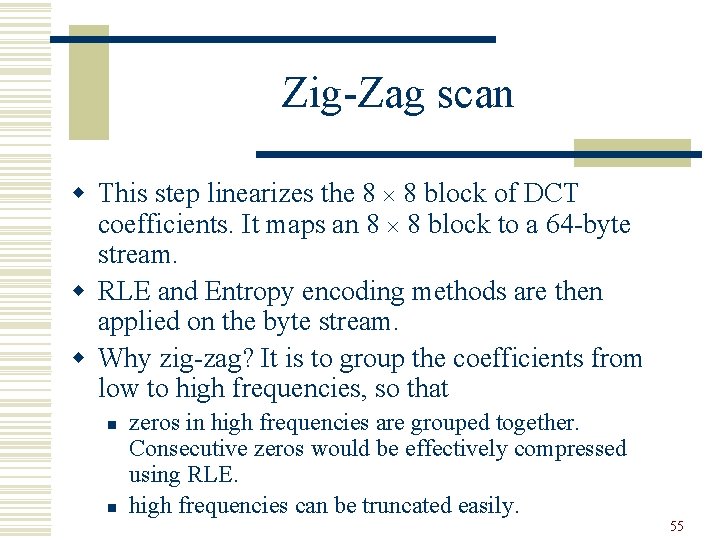
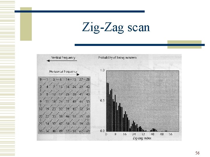
Zig-Zag scan w This step linearizes the 8 8 block of DCT coefficients. It maps an 8 8 block to a 64 -byte stream. w RLE and Entropy encoding methods are then applied on the byte stream. w Why zig-zag? It is to group the coefficients from low to high frequencies, so that n n zeros in high frequencies are grouped together. Consecutive zeros would be effectively compressed using RLE. high frequencies can be truncated easily. 55

Zig-Zag scan 56

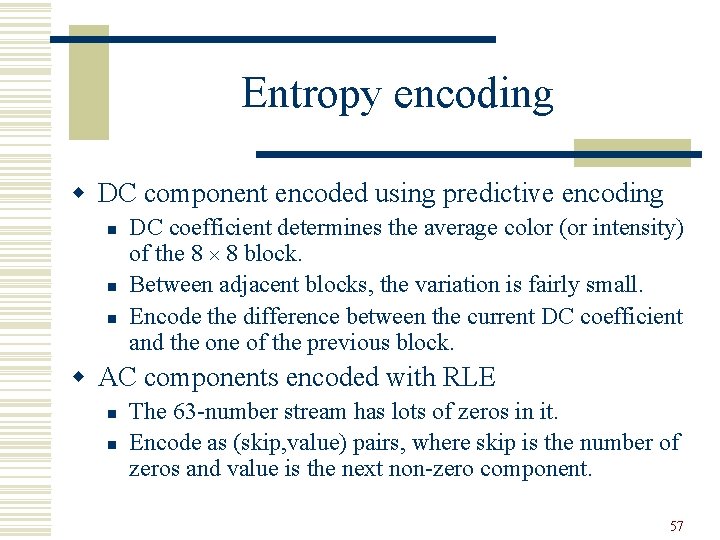
Entropy encoding w DC component encoded using predictive encoding n n n DC coefficient determines the average color (or intensity) of the 8 8 block. Between adjacent blocks, the variation is fairly small. Encode the difference between the current DC coefficient and the one of the previous block. w AC components encoded with RLE n n The 63 -number stream has lots of zeros in it. Encode as (skip, value) pairs, where skip is the number of zeros and value is the next non-zero component. 57

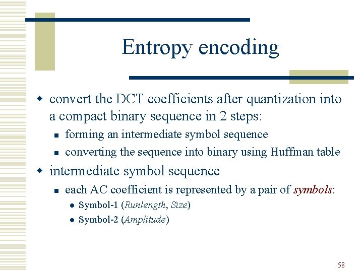
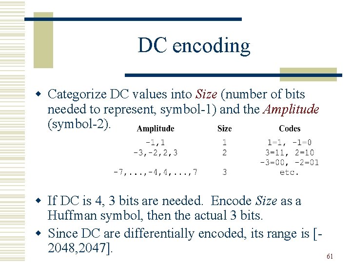
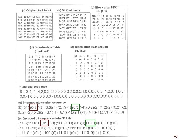
Entropy encoding w convert the DCT coefficients after quantization into a compact binary sequence in 2 steps: n n forming an intermediate symbol sequence converting the sequence into binary using Huffman table w intermediate symbol sequence n each AC coefficient is represented by a pair of symbols: l l Symbol-1 (Runlength, Size) Symbol-2 (Amplitude) 58

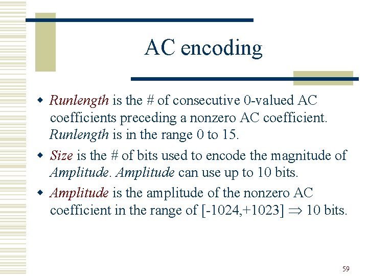
AC encoding w Runlength is the # of consecutive 0 -valued AC coefficients preceding a nonzero AC coefficient. Runlength is in the range 0 to 15. w Size is the # of bits used to encode the magnitude of Amplitude can use up to 10 bits. w Amplitude is the amplitude of the nonzero AC coefficient in the range of [-1024, +1023] 10 bits. 59

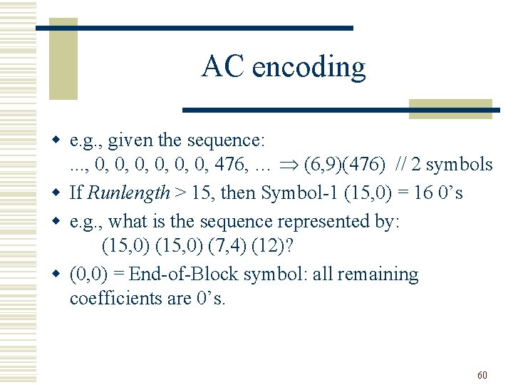
AC encoding w e. g. , given the sequence: . . . , 0, 0, 0, 476, … (6, 9)(476) // 2 symbols w If Runlength > 15, then Symbol-1 (15, 0) = 16 0’s w e. g. , what is the sequence represented by: (15, 0) (7, 4) (12)? w (0, 0) = End-of-Block symbol: all remaining coefficients are 0’s. 60

DC encoding w Categorize DC values into Size (number of bits needed to represent, symbol-1) and the Amplitude (symbol-2). w If DC is 4, 3 bits are needed. Encode Size as a Huffman symbol, then the actual 3 bits. w Since DC are differentially encoded, its range is [2048, 2047]. 61

62

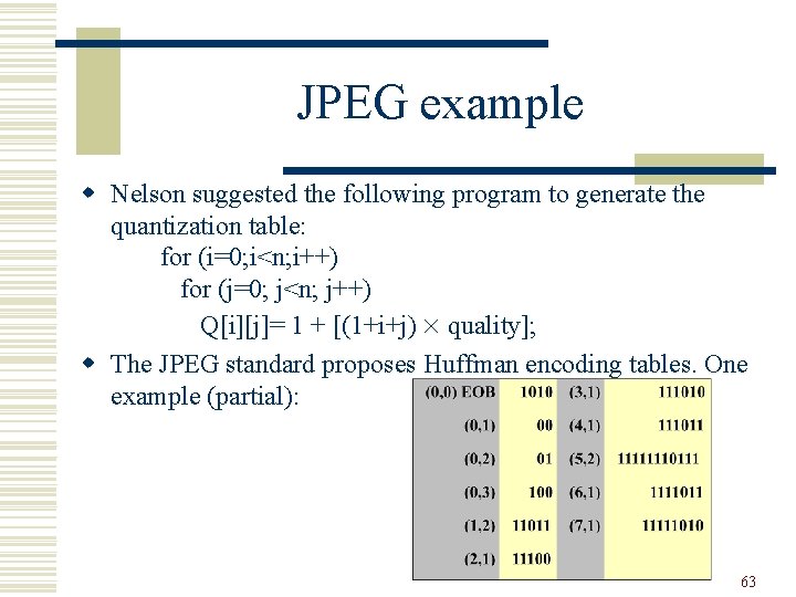
JPEG example w Nelson suggested the following program to generate the quantization table: for (i=0; i<n; i++) for (j=0; j<n; j++) Q[i][j]= 1 + [(1+i+j) quality]; w The JPEG standard proposes Huffman encoding tables. One example (partial): 63

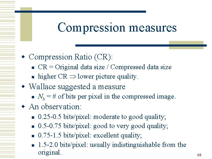
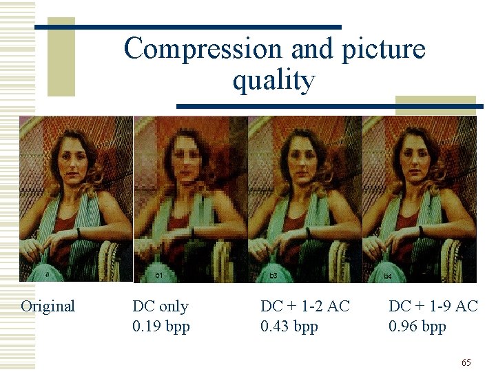
Compression measures w Compression Ratio (CR): n n CR = Original data size / Compressed data size higher CR lower picture quality. w Wallace suggested a measure n Nb = # of bits per pixel in the compressed image. w An observation: n n 0. 25 -0. 5 bits/pixel: moderate to good quality; 0. 5 -0. 75 bits/pixel: good to very good quality; 0. 75 -1. 5 bits/pixel: excellent quality; 1. 5 -2. 0 bits/pixel: usually indistinguishable from the original. 64

Compression and picture quality Original DC only 0. 19 bpp DC + 1 -2 AC 0. 43 bpp DC + 1 -9 AC 0. 96 bpp 65

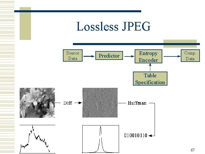
Lossless mode of JPEG compression w A special case of JPEG where there is no loss in the encoding process. w In this mode, image processing and quantization use a predictive technique instead of transformation encoding. w Neighboring pixels are taken as predictors, and the difference between the predicted and the actual values are encoded using Huffman methods. 66

Lossless JPEG Source Data Predictor Entropy Encoder Comp. Data Table Specification 67

Lossless JPEG w Normally, pixel values do not vary by much except at intensity (color) edges. The differences have small values in most regions of the image. Effective entropy compression is possible. 68

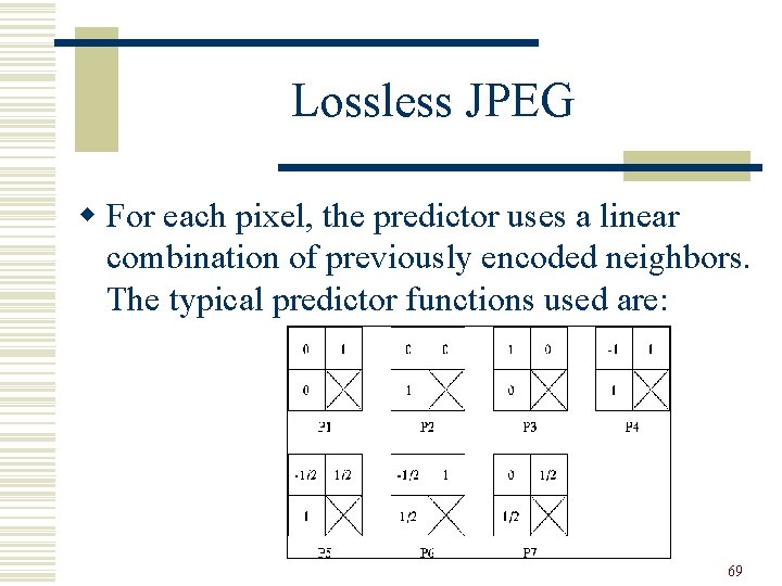
Lossless JPEG w For each pixel, the predictor uses a linear combination of previously encoded neighbors. The typical predictor functions used are: 69

Lossless JPEG w 2 D predictors (4 -7) usually do better than 1 D predictors. (P 0 is “no prediction”) w Typical compression ratio achieved is about 2: 1. 70

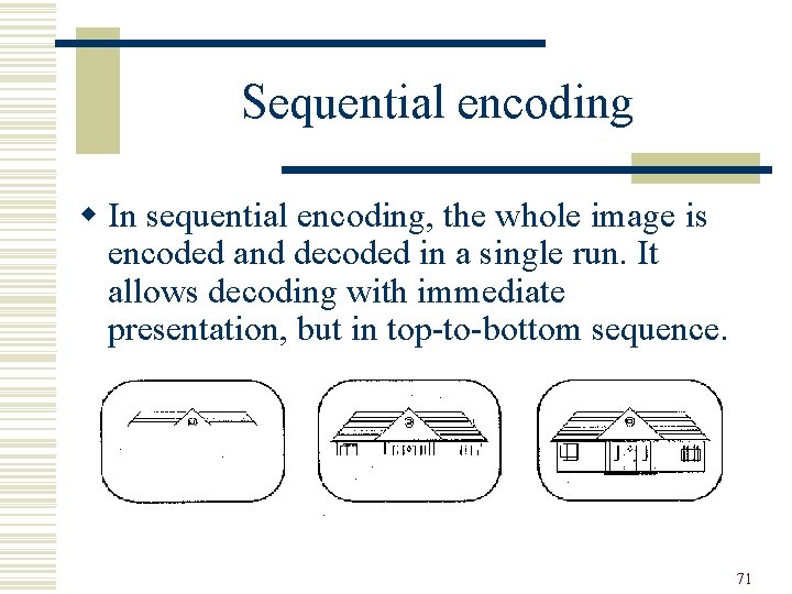
Sequential encoding w In sequential encoding, the whole image is encoded and decoded in a single run. It allows decoding with immediate presentation, but in top-to-bottom sequence. 71

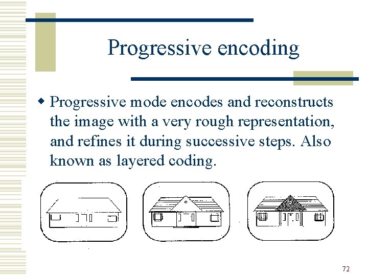
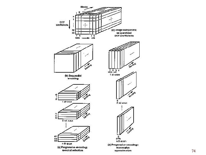
Progressive encoding w Progressive mode encodes and reconstructs the image with a very rough representation, and refines it during successive steps. Also known as layered coding. 72

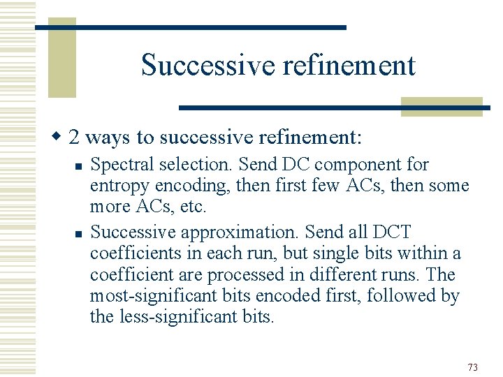
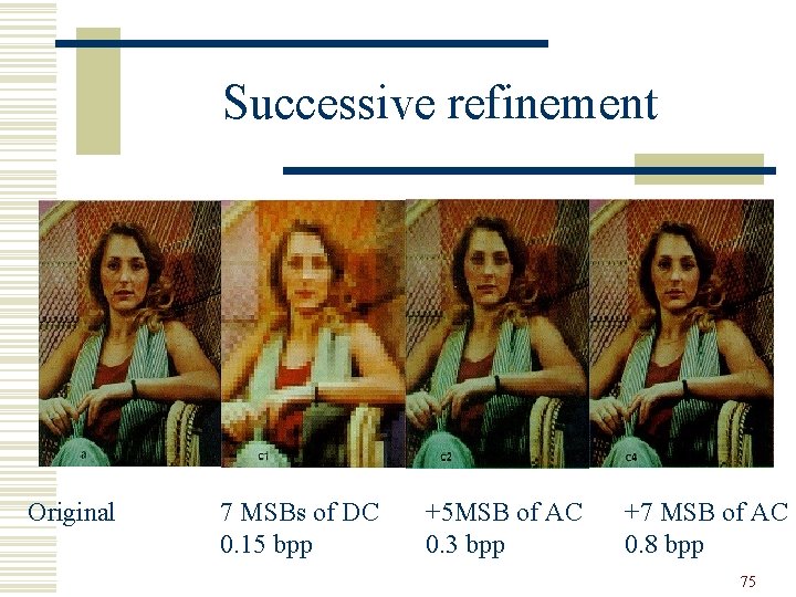
Successive refinement w 2 ways to successive refinement: n n Spectral selection. Send DC component for entropy encoding, then first few ACs, then some more ACs, etc. Successive approximation. Send all DCT coefficients in each run, but single bits within a coefficient are processed in different runs. The most-significant bits encoded first, followed by the less-significant bits. 73

74

Successive refinement Original 7 MSBs of DC 0. 15 bpp +5 MSB of AC 0. 3 bpp +7 MSB of AC 0. 8 bpp 75

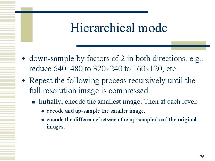
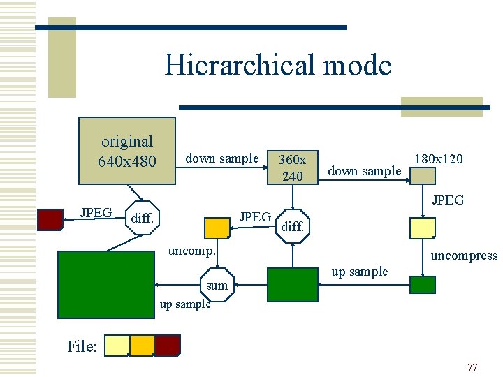
Hierarchical mode w down-sample by factors of 2 in both directions, e. g. , reduce 640 480 to 320 240 to 160 120, etc. w Repeat the following process recursively until the full resolution image is compressed. n Initially, encode the smallest image. Then at each level: l l decode and up-sample the smaller image. encode the difference between the up-sampled and the original images. 76

Hierarchical mode original 640 x 480 JPEG down sample 360 x 240 down sample 180 x 120 JPEG diff. uncomp. sum uncompress up sample File: 77

Hierarchical mode w Since the original image is encoded at different resolutions, n n it requires more storage for multiple resolutions. Advantage: the picture is immediately available at different resolutions. Scaling is cheap when display system works only with a lower resolution. 78

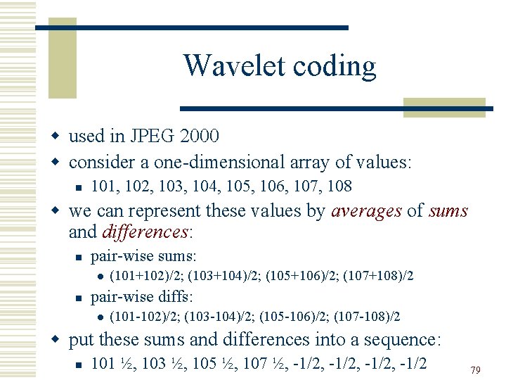
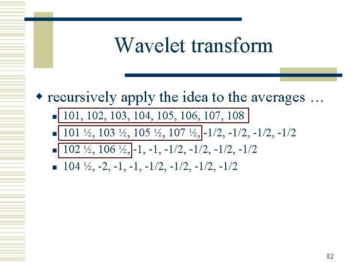
Wavelet coding w used in JPEG 2000 w consider a one-dimensional array of values: n 101, 102, 103, 104, 105, 106, 107, 108 w we can represent these values by averages of sums and differences: n pair-wise sums: l n (101+102)/2; (103+104)/2; (105+106)/2; (107+108)/2 pair-wise diffs: l (101 -102)/2; (103 -104)/2; (105 -106)/2; (107 -108)/2 w put these sums and differences into a sequence: n 101 ½, 103 ½, 105 ½, 107 ½, -1/2, -1/2 79

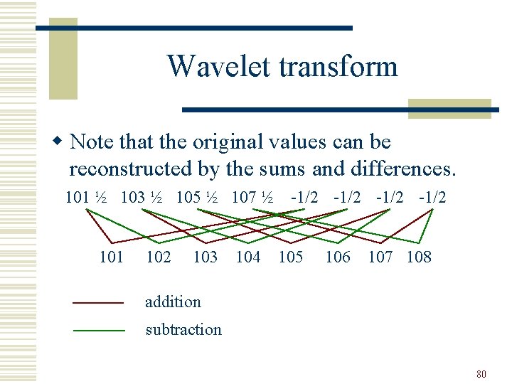
Wavelet transform w Note that the original values can be reconstructed by the sums and differences. 101 ½ 103 ½ 105 ½ 107 ½ 101 102 103 104 -1/2 105 106 107 108 addition subtraction 80

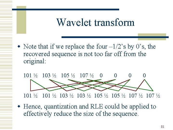
Wavelet transform w Note that if we replace the four – 1/2’s by 0’s, the recovered sequence is not too far off from the original: 101 ½ 103 ½ 105 ½ 107 ½ 0 0 101 ½ 103 ½ 105 ½ 107 ½ w Hence, quantization and RLE could be applied to effectively reduce the size of the sequence. 81

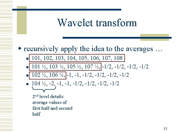
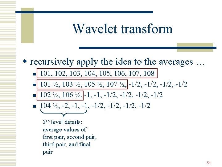
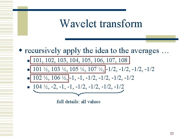
Wavelet transform w recursively apply the idea to the averages … n n 101, 102, 103, 104, 105, 106, 107, 108 101 ½, 103 ½, 105 ½, 107 ½, -1/2, -1/2 102 ½, 106 ½, -1, -1/2, -1/2 104 ½, -2, -1, -1/2, -1/2 82

Wavelet transform w recursively apply the idea to the averages … n n 101, 102, 103, 104, 105, 106, 107, 108 101 ½, 103 ½, 105 ½, 107 ½, -1/2, -1/2 102 ½, 106 ½, -1, -1/2, -1/2 104 ½, -2, -1, -1/2, -1/2 2 nd level details: average values of first half and second half 83

Wavelet transform w recursively apply the idea to the averages … n n 101, 102, 103, 104, 105, 106, 107, 108 101 ½, 103 ½, 105 ½, 107 ½, -1/2, -1/2 102 ½, 106 ½, -1, -1/2, -1/2 104 ½, -2, -1, -1/2, -1/2 3 rd level details: average values of first pair, second pair, third pair, and final pair 84

Wavelet transform w recursively apply the idea to the averages … n n 101, 102, 103, 104, 105, 106, 107, 108 101 ½, 103 ½, 105 ½, 107 ½, -1/2, -1/2 102 ½, 106 ½, -1, -1/2, -1/2 104 ½, -2, -1, -1/2, -1/2 full details: all values 85

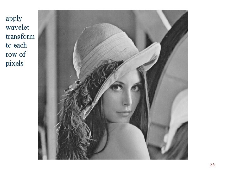
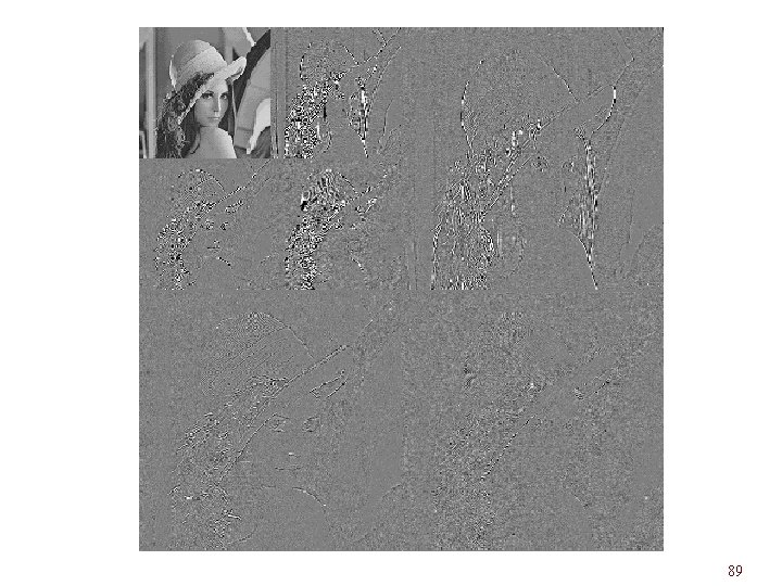
apply wavelet transform to each row of pixels 86

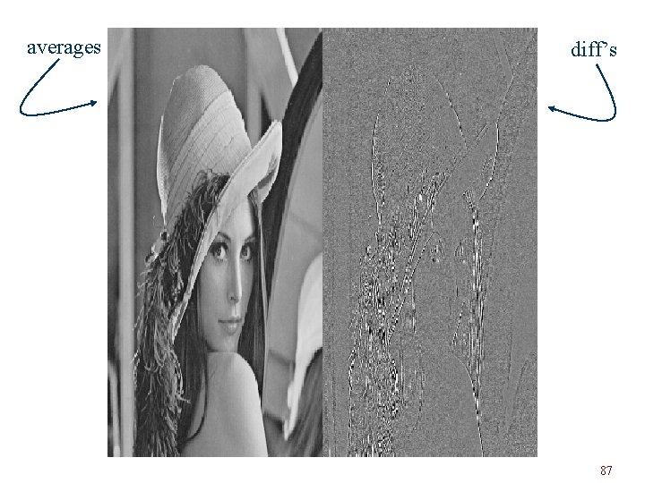
averages diff’s 87

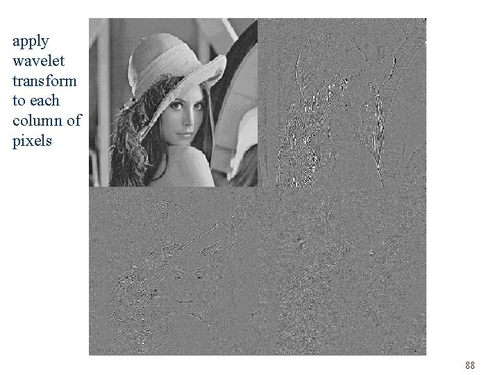
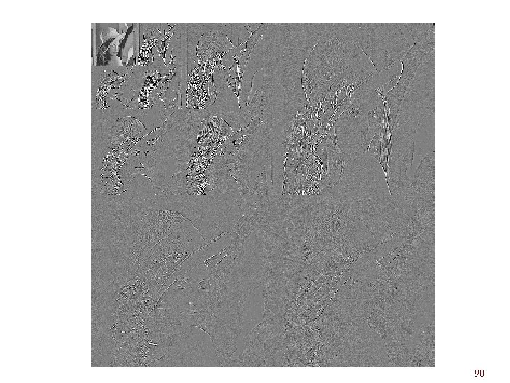
apply wavelet transform to each column of pixels 88

89

90

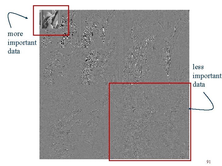
more important data less important data 91

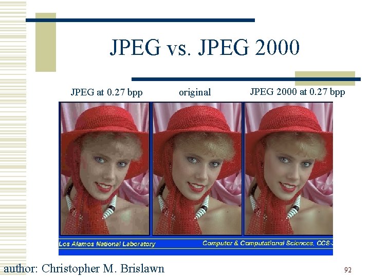
JPEG vs. JPEG 2000 JPEG at 0. 27 bpp author: Christopher M. Brislawn original JPEG 2000 at 0. 27 bpp 92

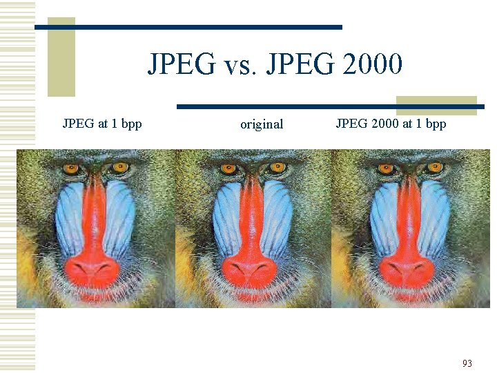
JPEG vs. JPEG 2000 JPEG at 1 bpp original JPEG 2000 at 1 bpp 93

JPEG vs. JPEG 2000 JPEG at 0. 5 bpp original JPEG 2000 at 0. 5 bpp 94