The LOCOI Lossless image Compression Algorithm Principles and

The LOCO-I Lossless image Compression Algorithm: Principles and Standardization into JPEG-LS Authors: M. J. Weinberger, G. Seroussi, G. Sapiro Source : IEEE Transactions on Image Processing, Vol. 9, No. 8, August 2000, 1309 -1324 Speaker: Chia-Chun Wu (吳佳駿) Date : 2004/10/20 NCHU 1

Outline 1. Introduction 2. Example 3. Modeler 4. Regular mode 5. Run mode 6. Coded data 7. Result 8. Conclusion 9. Comments NCHU 2

1. Introduction (1/2) LOCO-I (LOw COmplexity LOssless COmpression for Image) is the standard for lossless and near-lossless compression of continuous-tone images, such as JPEG-LS. NCHU 3

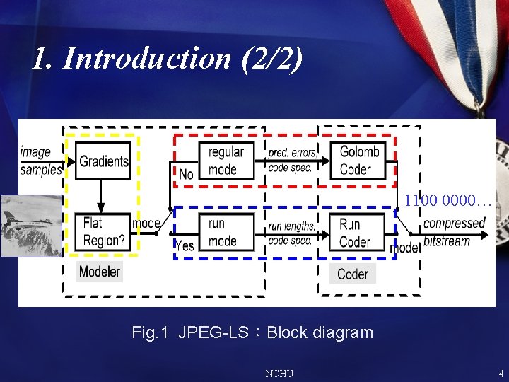
1. Introduction (2/2) 1100 0000… Fig. 1 JPEG-LS：Block diagram NCHU 4

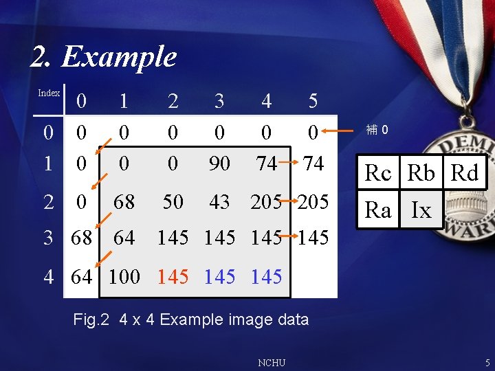
2. Example Index 0 1 0 0 2 0 0 3 0 90 4 0 74 5 0 74 2 0 68 50 43 205 補 0 Rc Rb Rd Ra Ix 3 68 64 145 145 4 64 100 145 145 Fig. 2 4 x 4 Example image data NCHU 5

3. Modeler 3. 1 Compute local gradients 3. 2 Local gradient quantization 3. 3 Quantized gradient merging 3. 4 Select the mode NCHU 6

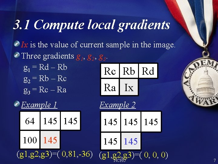
3. 1 Compute local gradients Ix is the value of current sample in the image. Three gradients g 1, g 2, g 3. g 1 = Rd – Rb Rc Rb Rd g 2 = Rb – Rc Ra Ix g 3 = Rc – Ra Example 1 Example 2 64 145 145 145 100 145 145 (g 1, g 2, g 3)=( 0, 81, -36) (g 1, g 2, g 3)=( 0, 0, 0) NCHU 7

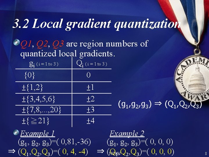
3. 2 Local gradient quantization Q 1, Q 2, Q 3 are region numbers of quantized local gradients. gi ( i = 1 to 3 ) Qi ( i = 1 to 3 ) {0} ±{1, 2} ±{3, 4, 5, 6} ±{7, 8, . . . , 20} ±{≧ 21} 0 ± 1 ± 2 ± 3 ± 4 (g 1, g 2, g 3) ⇒ (Q 1, Q 2, Q 3) Example 1 Example 2 (g 1, g 2, g 3)=( 0, 81, -36) (g 1, g 2, g 3)=( 0, 0, 0) ⇒ (Q 1, Q 2, Q 3)=( 0, 4, -4) ⇒ (Q NCHU 1, Q 2, Q 3)=( 0, 0, 0) 8

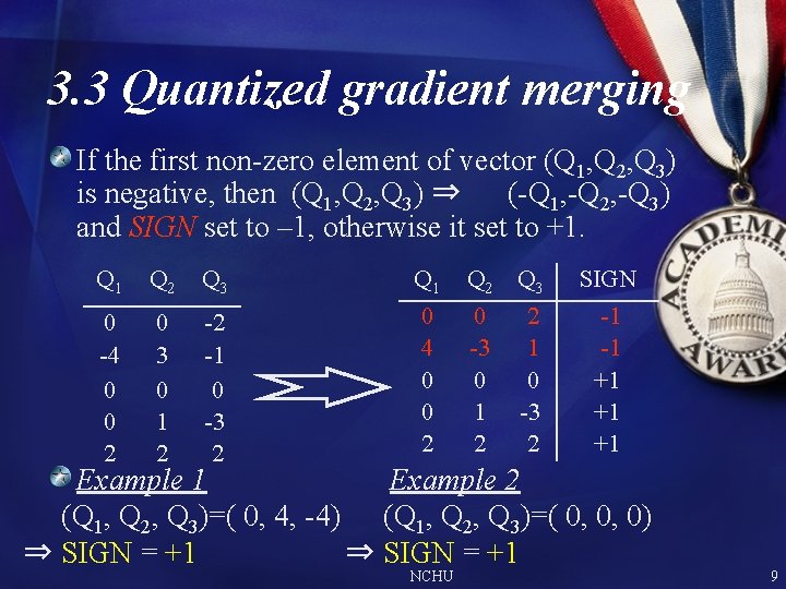
3. 3 Quantized gradient merging If the first non-zero element of vector (Q 1, Q 2, Q 3) is negative, then (Q 1, Q 2, Q 3) ⇒ (-Q 1, -Q 2, -Q 3) and SIGN set to – 1, otherwise it set to +1. Q 1 Q 2 Q 3 0 -4 0 0 2 0 3 0 1 2 -2 -1 0 -3 2 Q 1 0 4 0 0 2 Q 3 0 2 -3 1 0 0 1 -3 2 2 SIGN -1 -1 +1 +1 +1 Example 2 (Q 1, Q 2, Q 3)=( 0, 4, -4) (Q 1, Q 2, Q 3)=( 0, 0, 0) ⇒ SIGN = +1 NCHU 9

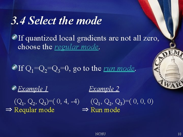
3. 4 Select the mode If quantized local gradients are not all zero, choose the regular mode. If Q 1=Q 2=Q 3=0, go to the run mode. Example 1 Example 2 (Q 1, Q 2, Q 3)=( 0, 4, -4) (Q 1, Q 2, Q 3)=( 0, 0, 0) ⇒ Reqular mode ⇒ Run mode NCHU 10

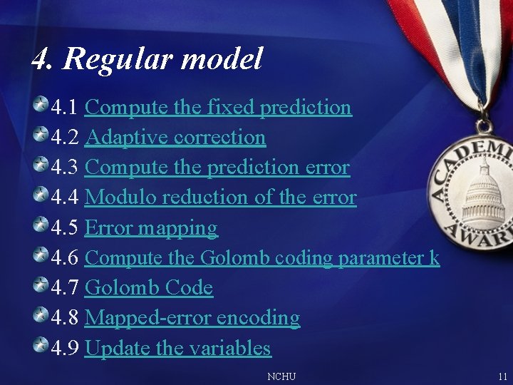
4. Regular model 4. 1 Compute the fixed prediction 4. 2 Adaptive correction 4. 3 Compute the prediction error 4. 4 Modulo reduction of the error 4. 5 Error mapping 4. 6 Compute the Golomb coding parameter k 4. 7 Golomb Code 4. 8 Mapped-error encoding 4. 9 Update the variables NCHU 11

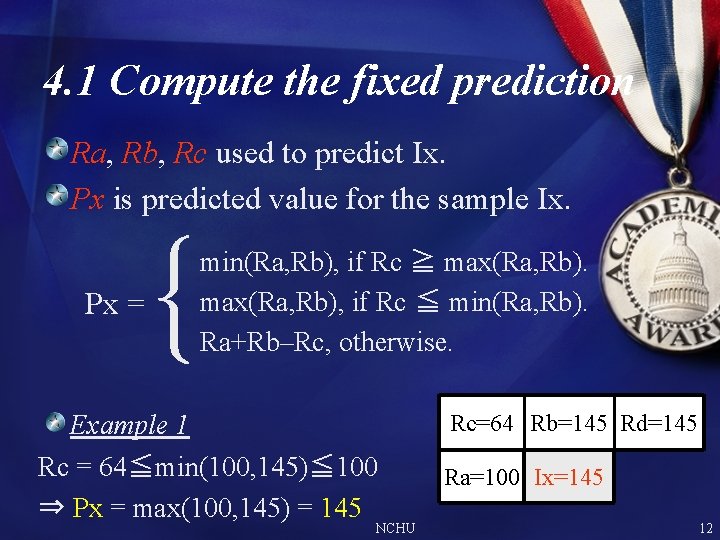
4. 1 Compute the fixed prediction Ra, Rb, Rc used to predict Ix. Px is predicted value for the sample Ix. { Px = min(Ra, Rb), if Rc ≧ max(Ra, Rb), if Rc ≦ min(Ra, Rb). Ra+Rb–Rc, otherwise. Example 1 Rc = 64≦min(100, 145)≦ 100 ⇒ Px = max(100, 145) = 145 NCHU Rc=64 Rb=145 Rd=145 Ra=100 Ix=145 12

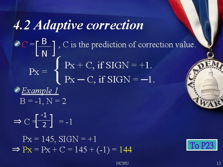
4. 2 Adaptive correction C= B N , C is the prediction of correction value. [ ] Px = { Px + C, if SIGN = +1. Px ─ C, if SIGN = ─1. Example 1 B = -1, N = 2 -1 2 [ ] = -1 ⇒C= Px = 145, SIGN = +1 ⇒ Px = Px + C = 145 + (-1) = 144 NCHU To P 23 13

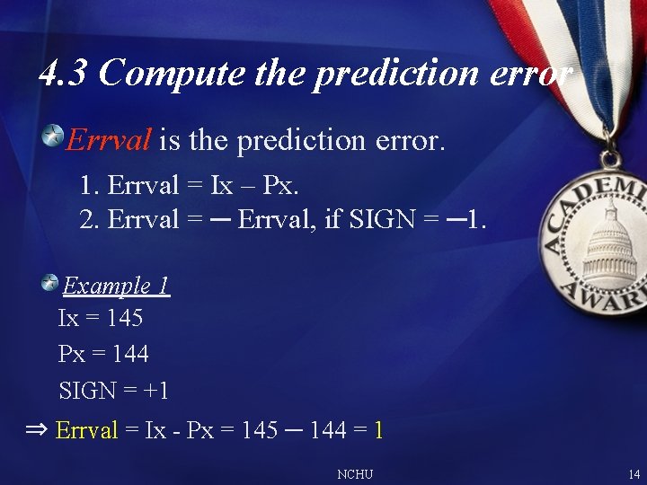
4. 3 Compute the prediction error Errval is the prediction error. 1. Errval = Ix – Px. 2. Errval = ─ Errval, if SIGN = ─1. Example 1 Ix = 145 Px = 144 SIGN = +1 ⇒ Errval = Ix - Px = 145 ─ 144 = 1 NCHU 14

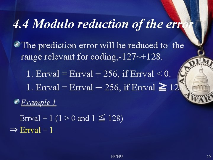
4. 4 Modulo reduction of the error The prediction error will be reduced to the range relevant for coding, -127~+128. 1. Errval = Errval + 256, if Errval < 0. 1. Errval = Errval ─ 256, if Errval ≧ 128. Example 1 Errval = 1 (1 > 0 and 1 ≦ 128) ⇒ Errval = 1 NCHU 15

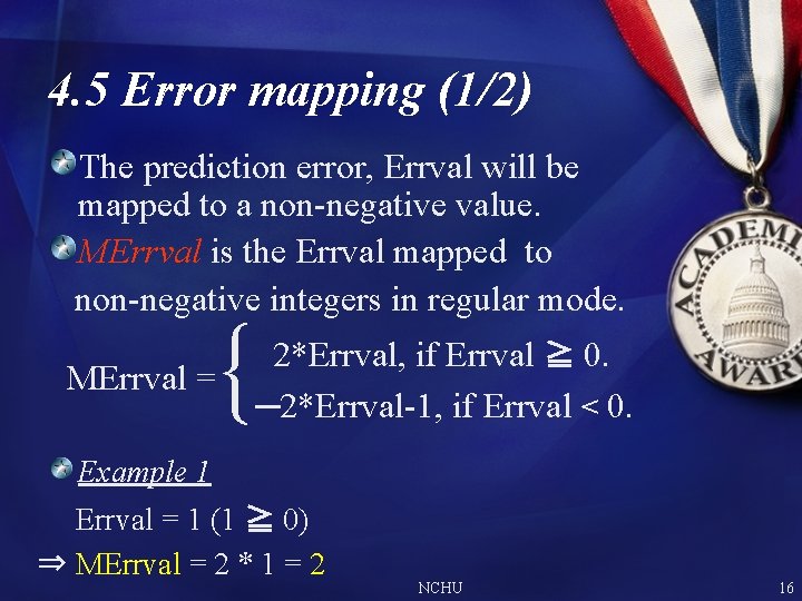
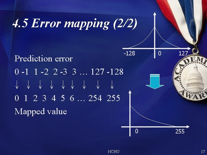
4. 5 Error mapping (1/2) The prediction error, Errval will be mapped to a non-negative value. MErrval is the Errval mapped to non-negative integers in regular mode. { MErrval = 2*Errval, if Errval ≧ 0. ─2*Errval-1, if Errval < 0. Example 1 Errval = 1 (1 ≧ 0) ⇒ MErrval = 2 * 1 = 2 NCHU 16

4. 5 Error mapping (2/2) -128 0 Prediction error 0 -1 1 -2 2 -3 3 … 127 -128 ↓ ↓ ↓↓ ↓ 0 1 2 3 4 5 6 … 254 255 Mapped value 0 NCHU 127 255 17

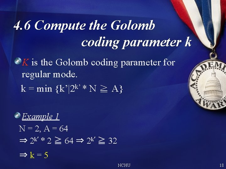
4. 6 Compute the Golomb coding parameter k K is the Golomb coding parameter for regular mode. k = min {k’|2 k’ * N ≧ A} Example 1 N = 2, A = 64 ⇒ 2 k’ * 2 ≧ 64 ⇒ 2 k’ ≧ 32 ⇒k=5 NCHU 18

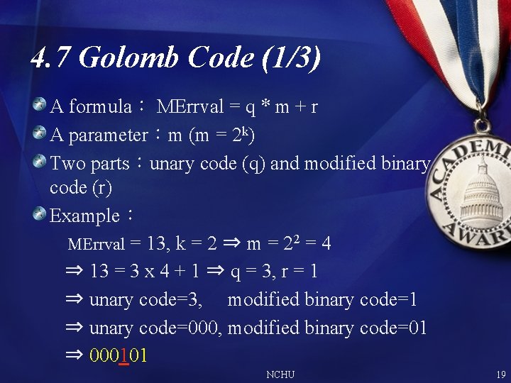
4. 7 Golomb Code (1/3) A formula： MErrval = q * m + r A parameter：m (m = 2 k) Two parts：unary code (q) and modified binary code (r) Example： MErrval = 13, k = 2 ⇒ m = 22 = 4 ⇒ 13 = 3 x 4 + 1 ⇒ q = 3, r = 1 ⇒ unary code=3, modified binary code=1 ⇒ unary code=000, modified binary code=01 ⇒ 000101 NCHU 19

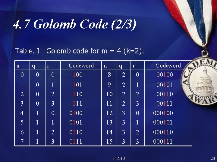
4. 7 Golomb Code (2/3) Table. Ⅰ Golomb code for m = 4 (k=2). n q r Codeword 0 0 0 100 8 2 0 00100 1 2 3 4 5 6 7 0 0 0 1 1 1 2 3 0 1 2 3 101 110 111 0100 0101 0110 0111 9 10 11 12 13 14 15 2 2 2 3 3 1 2 3 00101 00110 00111 000100 000101 000110 000111 NCHU 20

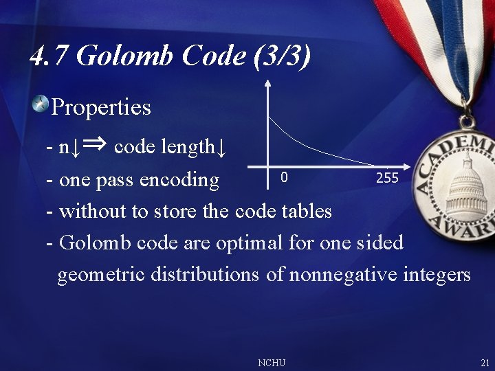
4. 7 Golomb Code (3/3) Properties - n↓⇒ code length↓ 0 255 - one pass encoding - without to store the code tables - Golomb code are optimal for one sided geometric distributions of nonnegative integers NCHU 21

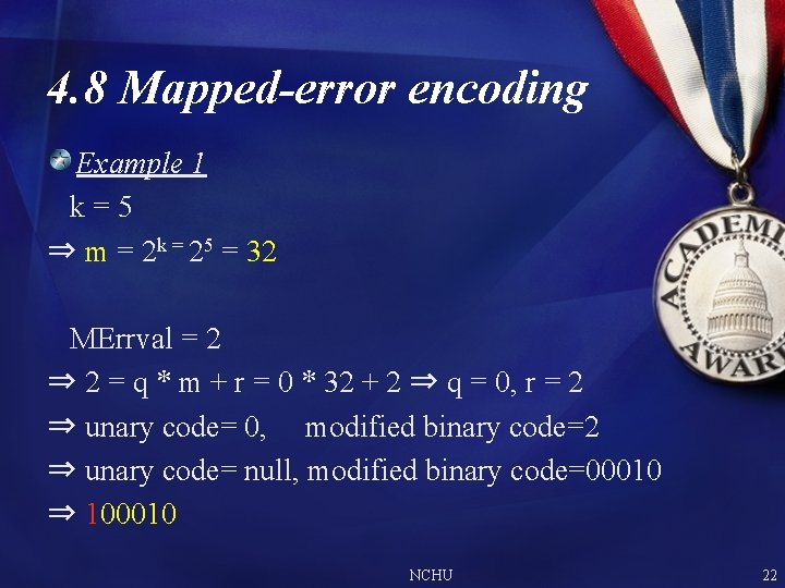
4. 8 Mapped-error encoding Example 1 k=5 ⇒ m = 2 k = 25 = 32 MErrval = 2 ⇒ 2 = q * m + r = 0 * 32 + 2 ⇒ q = 0, r = 2 ⇒ unary code= 0, modified binary code=2 ⇒ unary code= null, modified binary code=00010 ⇒ 100010 NCHU 22

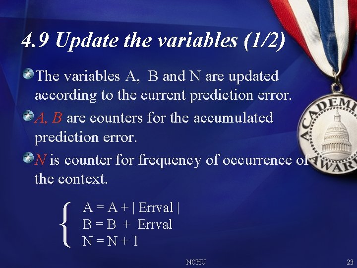
4. 9 Update the variables (1/2) The variables A, B and N are updated according to the current prediction error. A, B are counters for the accumulated prediction error. N is counter for frequency of occurrence of the context. { A = A + | Errval | B = B + Errval N=N+1 NCHU 23

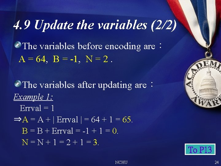
4. 9 Update the variables (2/2) The variables before encoding are： A = 64, B = -1, N = 2. The variables after updating are： Example 1: Errval = 1 ⇒A = A + | Errval | = 64 + 1 = 65. B = B + Errval = -1 + 1 = 0. N = N + 1 = 2 + 1 = 3. NCHU To P 13 24

5. Run model 5. 1 Run scanning 5. 2 Run-length coding NCHU 25

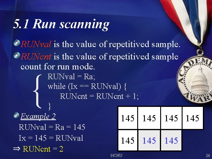
5. 1 Run scanning RUNval is the value of repetitived sample. RUNcnt is the value of repetitived sample count for run mode. RUNval = Ra; while (Ix == RUNval) { RUNcnt = RUNcnt + 1; } Example 2 145 145 RUNval = Ra = 145 Ix = 145 = RUNval 145 145 ⇒ RUNcnt = 2 { NCHU 26

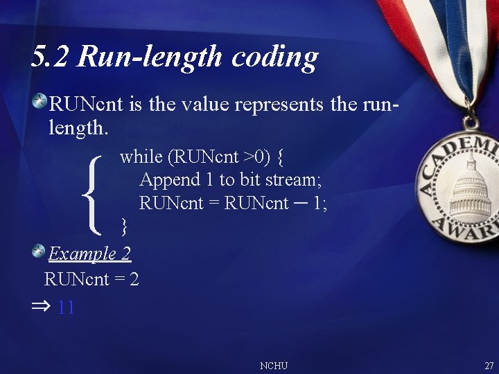
5. 2 Run-length coding RUNcnt is the value represents the runlength. while (RUNcnt >0) { Append 1 to bit stream; RUNcnt = RUNcnt ─ 1; } Example 2 RUNcnt = 2 ⇒ 11 { NCHU 27

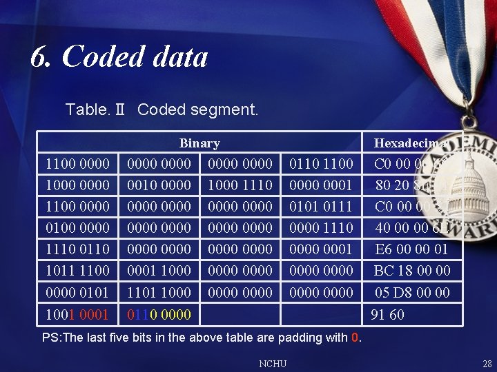
6. Coded data Table. Ⅱ Coded segment. Binary 1100 0000 1000 0000 1100 0000 0100 0000 1110 0110 1011 1100 0000 0101 1001 0000 0010 0000 0000 0001 1000 1101 1000 0110 0000 Hexadecimal 0000 1000 1110 0000 0000 0000 0110 1100 0001 0111 0000 1110 0001 0000 C 0 00 00 6 C 80 20 8 E 01 C 0 00 00 57 40 00 00 6 E E 6 00 00 01 BC 18 00 00 05 D 8 00 00 91 60 PS: The last five bits in the above table are padding with 0. NCHU 28

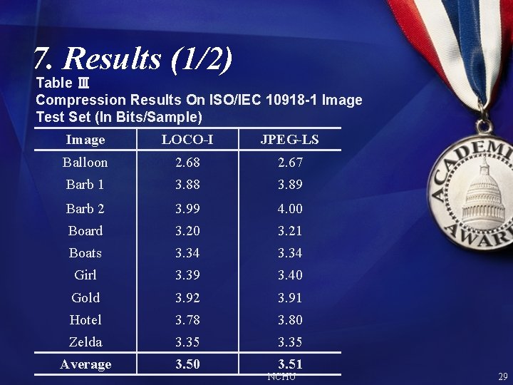
7. Results (1/2) Table Ⅲ Compression Results On ISO/IEC 10918 -1 Image Test Set (In Bits/Sample) Image LOCO-I JPEG-LS Balloon 2. 68 2. 67 Barb 1 3. 88 3. 89 Barb 2 3. 99 4. 00 Board 3. 20 3. 21 Boats 3. 34 Girl 3. 39 3. 40 Gold 3. 92 3. 91 Hotel 3. 78 3. 80 Zelda 3. 35 Average 3. 50 3. 51 NCHU 29

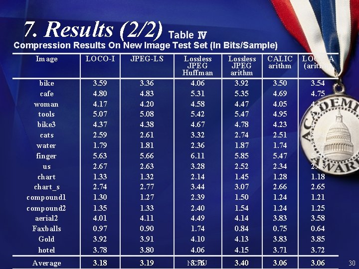
7. Results (2/2) Table Ⅳ Compression Results On New Image Test Set (In Bits/Sample) Image LOCO-I JPEG-LS Lossless JPEG arithm 3. 92 5. 35 4. 47 5. 47 4. 78 2. 74 1. 87 5. 85 2. 52 1. 45 3. 07 1. 50 1. 54 4. 14 0. 84 4. 13 4. 15 CALIC arithm LOCO-A (arithm) 3. 36 4. 83 4. 20 5. 08 4. 38 2. 61 1. 81 5. 66 2. 63 1. 32 2. 77 1. 27 1. 33 4. 11 0. 90 3. 91 3. 80 Lossless JPEG Huffman 4. 06 5. 31 4. 58 5. 42 4. 67 3. 32 2. 36 6. 11 3. 28 2. 14 3. 44 2. 39 2. 40 4. 49 1. 74 4. 10 4. 06 bike cafe woman tools bike 3 cats water finger us chart_s compound 1 compound 2 aerial 2 Faxballs Gold hotel 3. 59 4. 80 4. 17 5. 07 4. 37 2. 59 1. 79 5. 63 2. 67 1. 33 2. 74 1. 30 1. 35 4. 01 0. 97 3. 92 3. 78 3. 50 4. 69 4. 05 4. 95 4. 23 2. 51 1. 74 5. 47 2. 34 1. 28 2. 66 1. 24 3. 83 0. 75 3. 83 3. 71 3. 54 4. 75 4. 11 5. 01 4. 33 2. 54 1. 75 5. 50 2. 45 1. 18 2. 65 1. 21 1. 25 3. 58 0. 64 3. 85 3. 72 Average 3. 18 3. 19 3. 76 NCHU 3. 40 3. 06 30

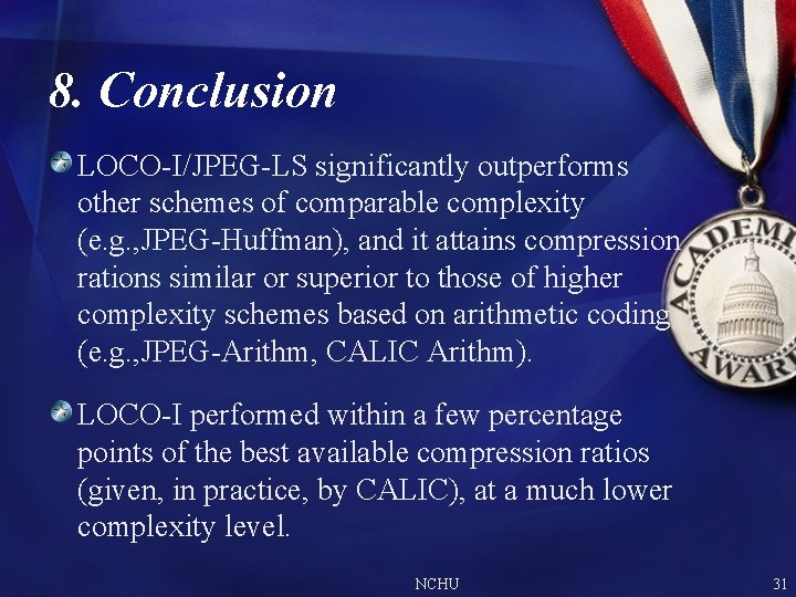
8. Conclusion LOCO-I/JPEG-LS significantly outperforms other schemes of comparable complexity (e. g. , JPEG-Huffman), and it attains compression rations similar or superior to those of higher complexity schemes based on arithmetic coding (e. g. , JPEG-Arithm, CALIC Arithm). LOCO-I performed within a few percentage points of the best available compression ratios (given, in practice, by CALIC), at a much lower complexity level. NCHU 31

The end Thank you!! NCHU 33