Chapter 14 Applications of Linear Optimization Applications of

Chapter 14 Applications of Linear Optimization

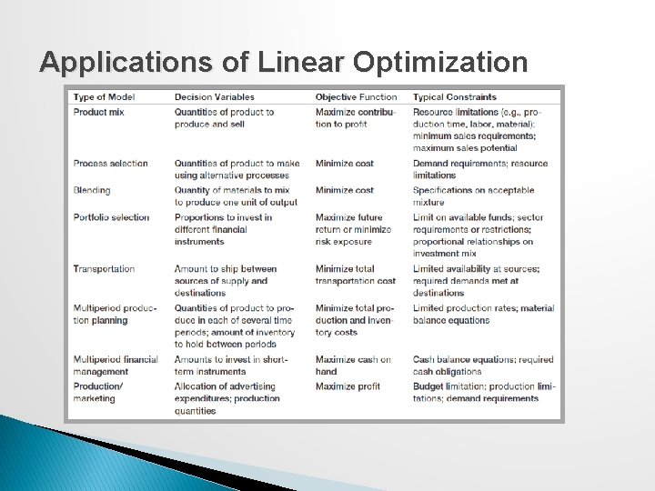
Applications of Linear Optimization

Building Linear Optimization Models Building optimization models is more of an art than a science. ◦ Learning how to build models requires logical thought facilitated by studying examples and observing their characteristics. Key issues: ◦ ◦ ◦ Formulation Spreadsheet implementation Interpreting results Scenario and sensitivity analysis Gaining insight for making good decisions

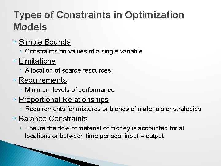
Types of Constraints in Optimization Models Simple Bounds ◦ Constraints on values of a single variable Limitations ◦ Allocation of scarce resources Requirements ◦ Minimum levels of performance Proportional Relationships ◦ Requirements for mixtures or blends of materials or strategies Balance Constraints ◦ Ensure the flow of material or money is accounted for at locations or between time periods: input = output

Process Selection Models Process selection models generally involve choosing among different types of processes to produce a good. ◦ Example: make or buy decisions

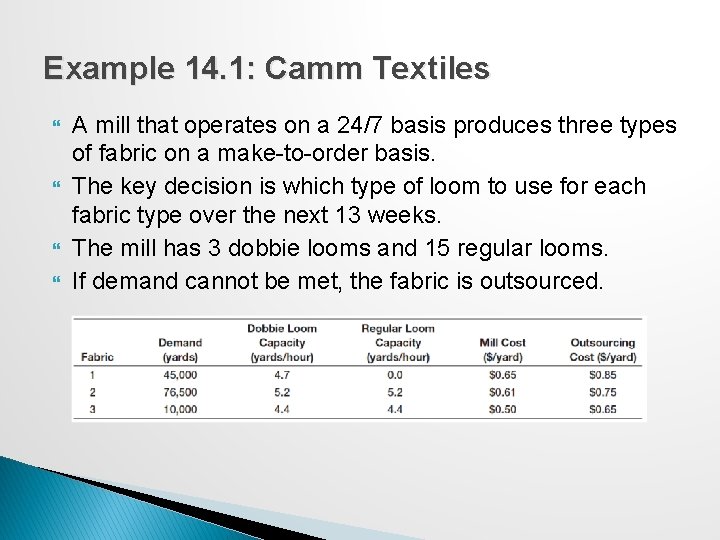
Example 14. 1: Camm Textiles A mill that operates on a 24/7 basis produces three types of fabric on a make-to-order basis. The key decision is which type of loom to use for each fabric type over the next 13 weeks. The mill has 3 dobbie looms and 15 regular looms. If demand cannot be met, the fabric is outsourced.

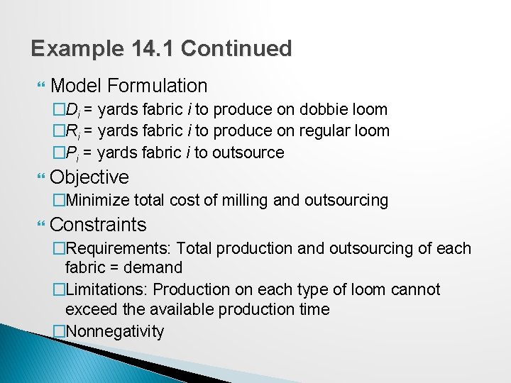
Example 14. 1 Continued Model Formulation �Di = yards fabric i to produce on dobbie loom �Ri = yards fabric i to produce on regular loom �Pi = yards fabric i to outsource Objective �Minimize total cost of milling and outsourcing Constraints �Requirements: Total production and outsourcing of each fabric = demand �Limitations: Production on each type of loom cannot exceed the available production time �Nonnegativity

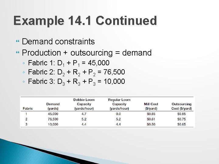
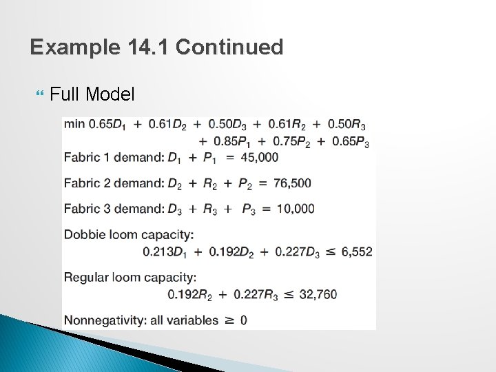
Example 14. 1 Continued Demand constraints Production + outsourcing = demand ◦ Fabric 1: D 1 + P 1 = 45, 000 ◦ Fabric 2: D 2 + R 2 + P 2 = 76, 500 ◦ Fabric 3: D 3 + R 3 + P 3 = 10, 000

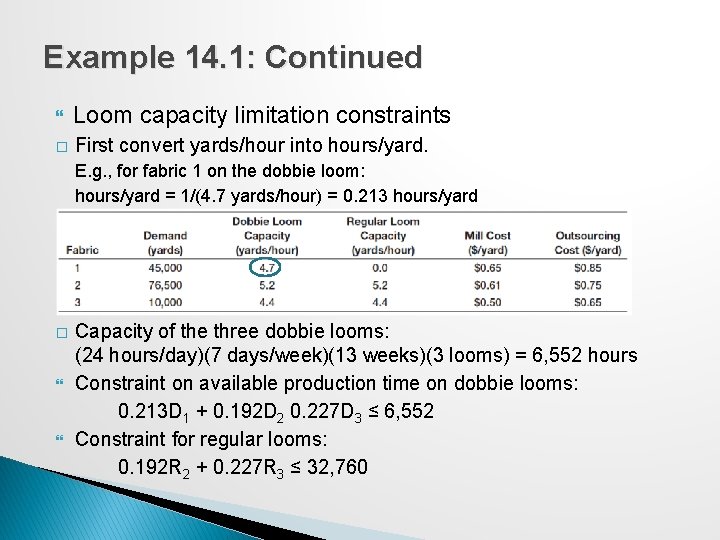
Example 14. 1: Continued Loom capacity limitation constraints � First convert yards/hour into hours/yard. E. g. , for fabric 1 on the dobbie loom: hours/yard = 1/(4. 7 yards/hour) = 0. 213 hours/yard � Capacity of the three dobbie looms: (24 hours/day)(7 days/week)(13 weeks)(3 looms) = 6, 552 hours Constraint on available production time on dobbie looms: 0. 213 D 1 + 0. 192 D 2 0. 227 D 3 ≤ 6, 552 Constraint for regular looms: 0. 192 R 2 + 0. 227 R 3 ≤ 32, 760

Example 14. 1 Continued Full Model

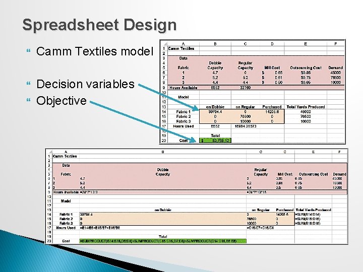
Spreadsheet Design Camm Textiles model Decision variables Objective

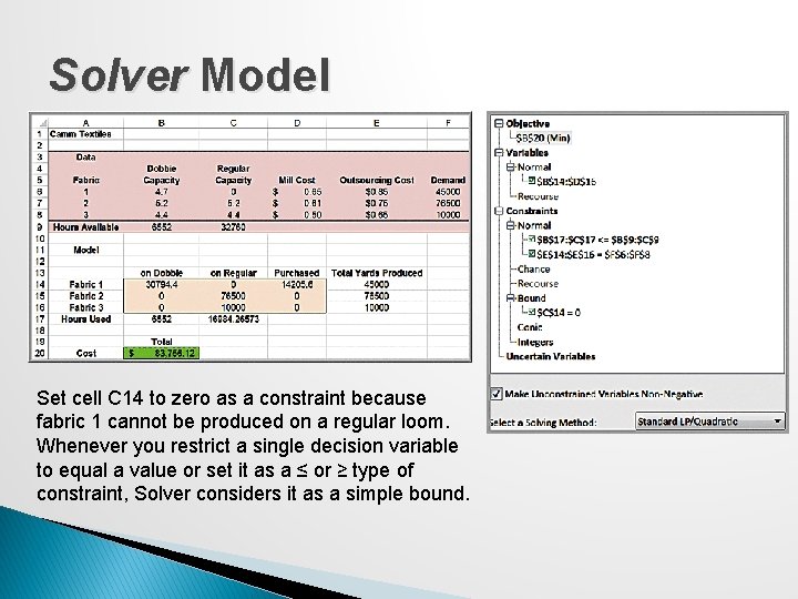
Solver Model Set cell C 14 to zero as a constraint because fabric 1 cannot be produced on a regular loom. Whenever you restrict a single decision variable to equal a value or set it as a ≤ or ≥ type of constraint, Solver considers it as a simple bound.

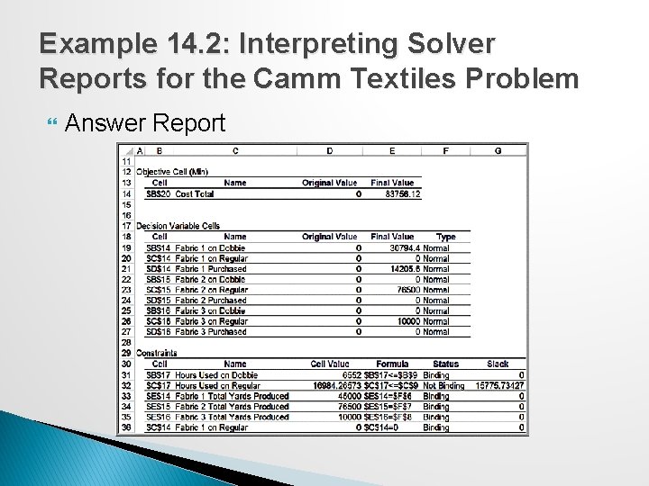
Example 14. 2: Interpreting Solver Reports for the Camm Textiles Problem Answer Report

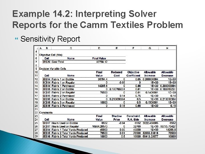
Example 14. 2: Interpreting Solver Reports for the Camm Textiles Problem Sensitivity Report

Solver Output and Data Visualization Solver requires some technical knowledge of linear optimization concepts and terminology, such as reduced costs and shadow prices. Data visualization can help analysts present optimization results in forms that are more understandable and can be easily explained to managers and clients in a report or presentation.

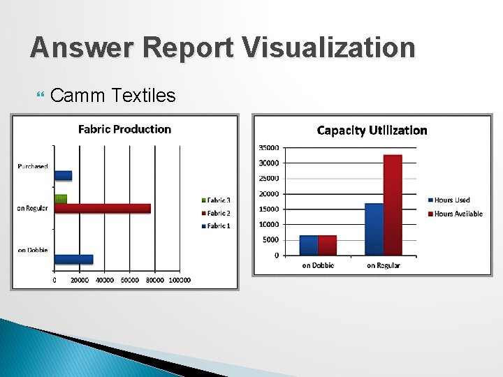
Answer Report Visualization Camm Textiles

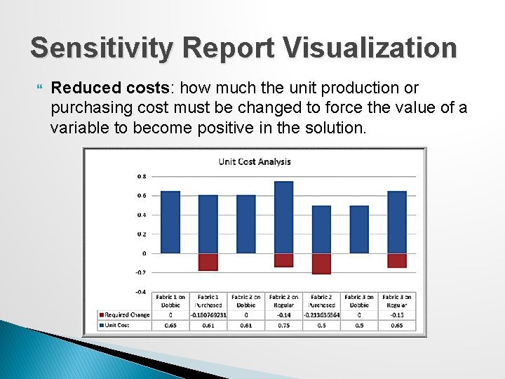
Sensitivity Report Visualization Reduced costs: how much the unit production or purchasing cost must be changed to force the value of a variable to become positive in the solution.

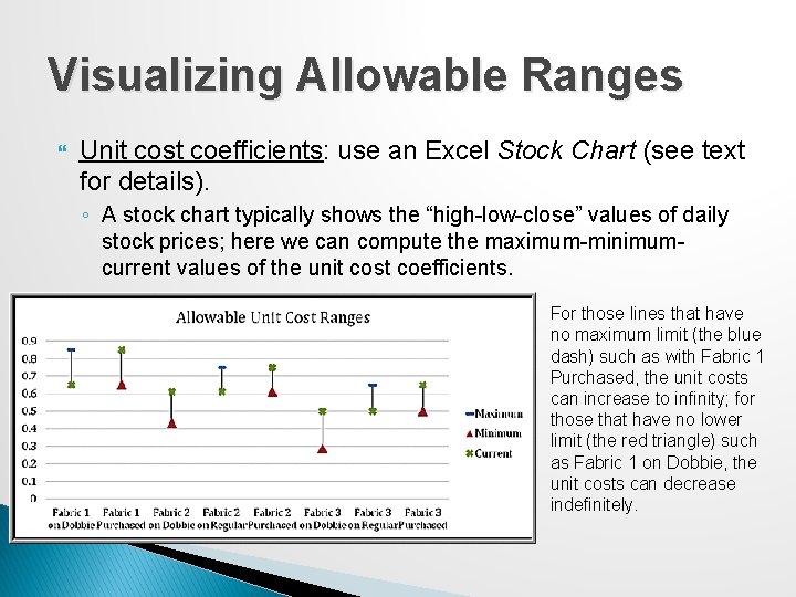
Visualizing Allowable Ranges Unit cost coefficients: use an Excel Stock Chart (see text for details). ◦ A stock chart typically shows the “high-low-close” values of daily stock prices; here we can compute the maximum-minimumcurrent values of the unit cost coefficients. For those lines that have no maximum limit (the blue dash) such as with Fabric 1 Purchased, the unit costs can increase to infinity; for those that have no lower limit (the red triangle) such as Fabric 1 on Dobbie, the unit costs can decrease indefinitely.

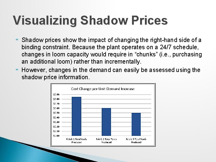
Visualizing Shadow Prices Shadow prices show the impact of changing the right-hand side of a binding constraint. Because the plant operates on a 24/7 schedule, changes in loom capacity would require in “chunks” (i. e. , purchasing an additional loom) rather than incrementally. However, changes in the demand can easily be assessed using the shadow price information.

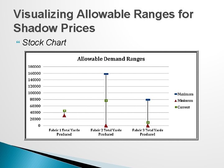
Visualizing Allowable Ranges for Shadow Prices Stock Chart

Blending Models Blending problems involve mixing several raw materials that have different characteristics to make a product that meets certain specifications. ◦ Dietary planning, gasoline and oil refining, coal and fertilizer production, and the production of many other types of bulk commodities involve blending. We typically see proportional constraints in blending models.

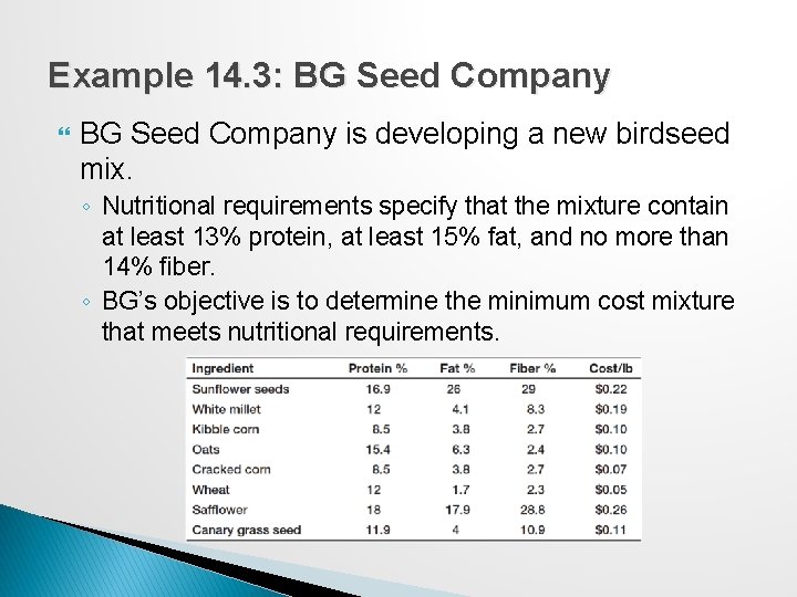
Example 14. 3: BG Seed Company is developing a new birdseed mix. ◦ Nutritional requirements specify that the mixture contain at least 13% protein, at least 15% fat, and no more than 14% fiber. ◦ BG’s objective is to determine the minimum cost mixture that meets nutritional requirements.

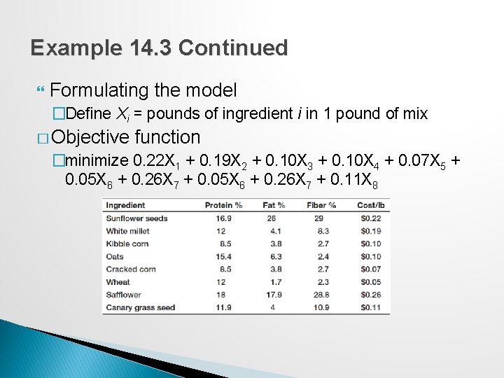
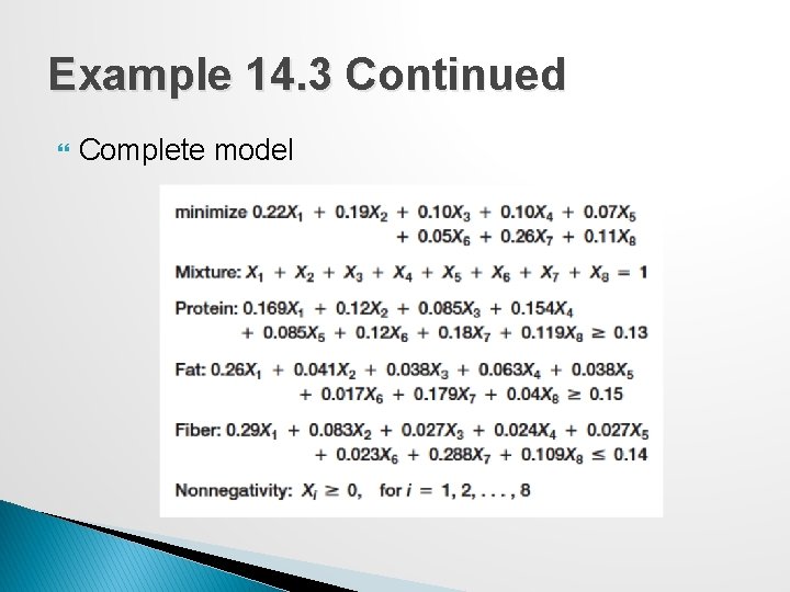
Example 14. 3 Continued Formulating the model �Define Xi = pounds of ingredient i in 1 pound of mix � Objective function �minimize 0. 22 X 1 + 0. 19 X 2 + 0. 10 X 3 + 0. 10 X 4 + 0. 07 X 5 + 0. 05 X 6 + 0. 26 X 7 + 0. 11 X 8

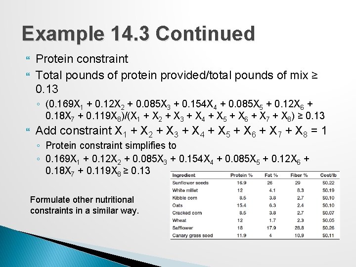
Example 14. 3 Continued Protein constraint Total pounds of protein provided/total pounds of mix ≥ 0. 13 ◦ (0. 169 X 1 + 0. 12 X 2 + 0. 085 X 3 + 0. 154 X 4 + 0. 085 X 5 + 0. 12 X 6 + 0. 18 X 7 + 0. 119 X 8)/(X 1 + X 2 + X 3 + X 4 + X 5 + X 6 + X 7 + X 8) ≥ 0. 13 Add constraint X 1 + X 2 + X 3 + X 4 + X 5 + X 6 + X 7 + X 8 = 1 ◦ Protein constraint simplifies to ◦ 0. 169 X 1 + 0. 12 X 2 + 0. 085 X 3 + 0. 154 X 4 + 0. 085 X 5 + 0. 12 X 6 + 0. 18 X 7 + 0. 119 X 8 ≥ 0. 13 Formulate other nutritional constraints in a similar way.

Example 14. 3 Continued Complete model

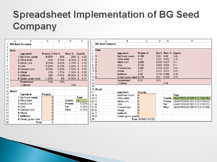
Spreadsheet Implementation of BG Seed Company

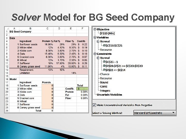
Solver Model for BG Seed Company

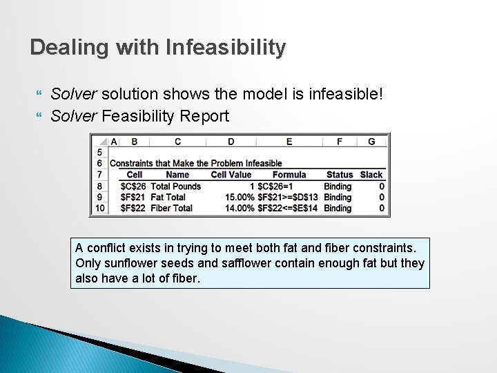
Dealing with Infeasibility Solver solution shows the model is infeasible! Solver Feasibility Report A conflict exists in trying to meet both fat and fiber constraints. Only sunflower seeds and safflower contain enough fat but they also have a lot of fiber.

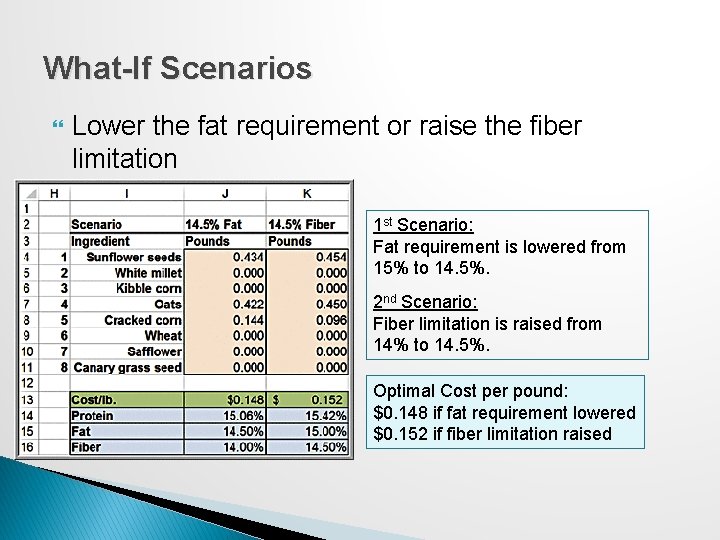
What-If Scenarios Lower the fat requirement or raise the fiber limitation 1 st Scenario: Fat requirement is lowered from 15% to 14. 5%. 2 nd Scenario: Fiber limitation is raised from 14% to 14. 5%. Optimal Cost per pound: $0. 148 if fat requirement lowered $0. 152 if fiber limitation raised

Portfolio Investment Models Many types of financial investment problems are modeled and solved using linear optimization. Such portfolio investment models problems have the basic characteristics of blending models.

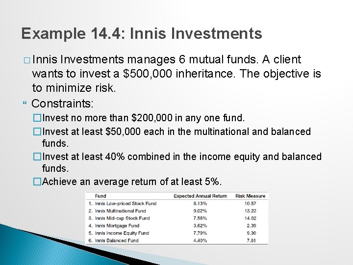
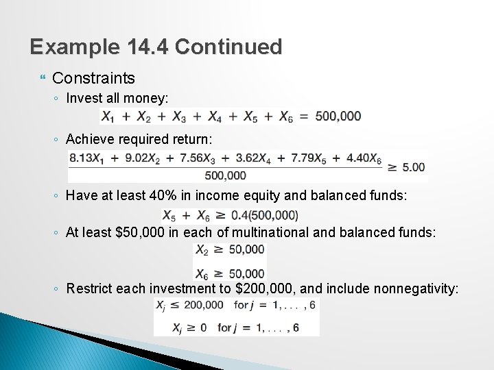
Example 14. 4: Innis Investments � Innis Investments manages 6 mutual funds. A client wants to invest a $500, 000 inheritance. The objective is to minimize risk. Constraints: �Invest no more than $200, 000 in any one fund. �Invest at least $50, 000 each in the multinational and balanced funds. �Invest at least 40% combined in the income equity and balanced funds. �Achieve an average return of at least 5%.

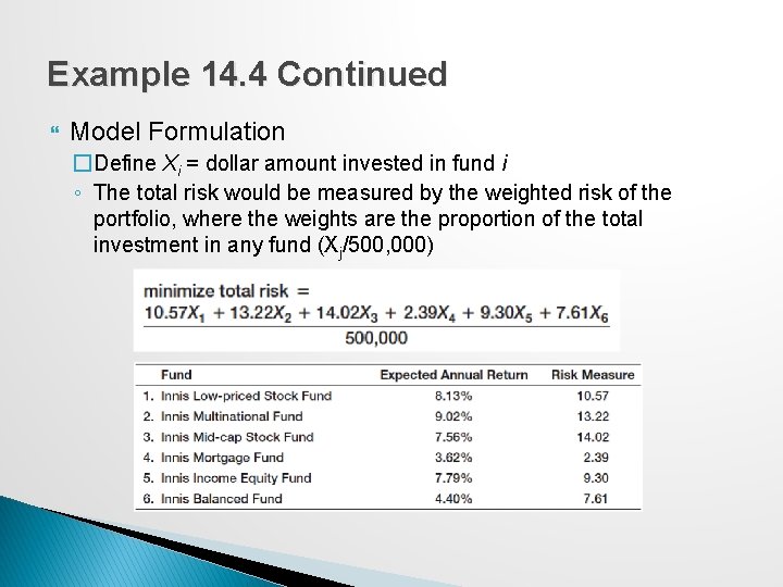
Example 14. 4 Continued Model Formulation �Define Xi = dollar amount invested in fund i ◦ The total risk would be measured by the weighted risk of the portfolio, where the weights are the proportion of the total investment in any fund (Xj/500, 000)

Example 14. 4 Continued Constraints ◦ Invest all money: ◦ Achieve required return: ◦ Have at least 40% in income equity and balanced funds: ◦ At least $50, 000 in each of multinational and balanced funds: ◦ Restrict each investment to $200, 000, and include nonnegativity:

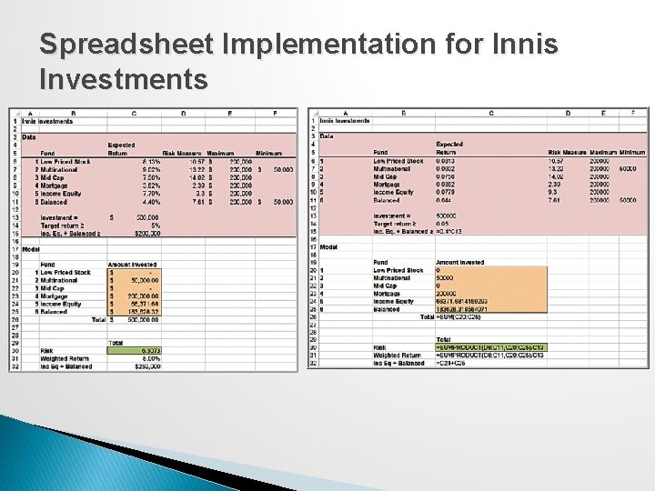
Spreadsheet Implementation for Innis Investments

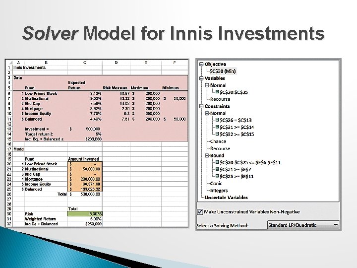
Solver Model for Innis Investments

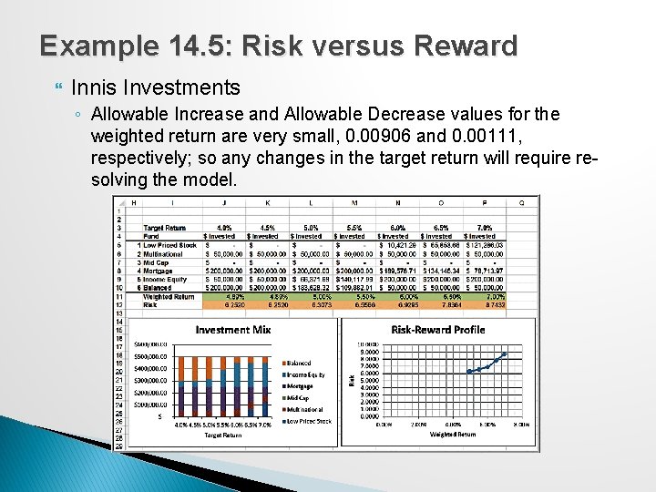
Example 14. 5: Risk versus Reward Innis Investments ◦ Allowable Increase and Allowable Decrease values for the weighted return are very small, 0. 00906 and 0. 00111, respectively; so any changes in the target return will require resolving the model.

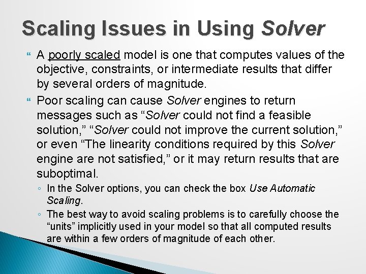
Scaling Issues in Using Solver A poorly scaled model is one that computes values of the objective, constraints, or intermediate results that differ by several orders of magnitude. Poor scaling can cause Solver engines to return messages such as “Solver could not find a feasible solution, ” “Solver could not improve the current solution, ” or even “The linearity conditions required by this Solver engine are not satisfied, ” or it may return results that are suboptimal. ◦ In the Solver options, you can check the box Use Automatic Scaling. ◦ The best way to avoid scaling problems is to carefully choose the “units” implicitly used in your model so that all computed results are within a few orders of magnitude of each other.

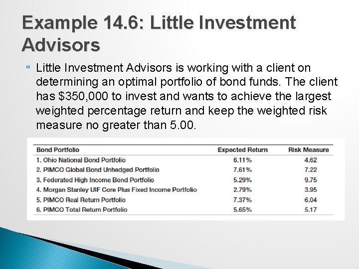
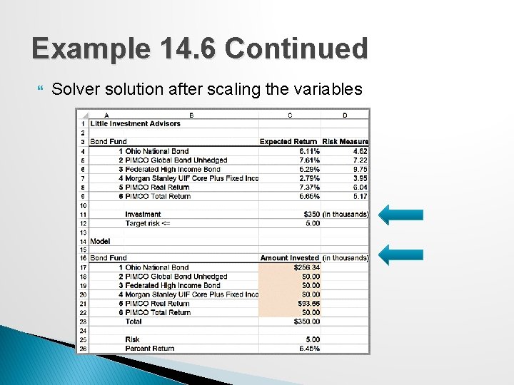
Example 14. 6: Little Investment Advisors is working with a client on determining an optimal portfolio of bond funds. The client has $350, 000 to invest and wants to achieve the largest weighted percentage return and keep the weighted risk measure no greater than 5. 00.

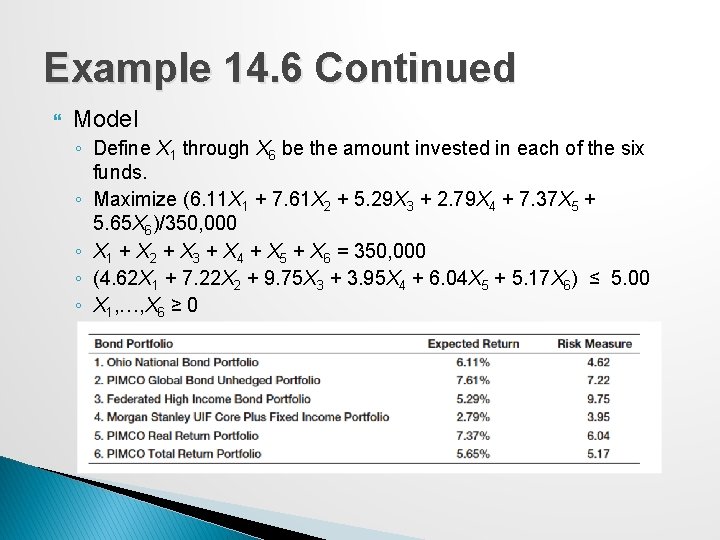
Example 14. 6 Continued Model ◦ Define X 1 through X 6 be the amount invested in each of the six funds. ◦ Maximize (6. 11 X 1 + 7. 61 X 2 + 5. 29 X 3 + 2. 79 X 4 + 7. 37 X 5 + 5. 65 X 6)/350, 000 ◦ X 1 + X 2 + X 3 + X 4 + X 5 + X 6 = 350, 000 ◦ (4. 62 X 1 + 7. 22 X 2 + 9. 75 X 3 + 3. 95 X 4 + 6. 04 X 5 + 5. 17 X 6) ≤ 5. 00 ◦ X 1, …, X 6 ≥ 0

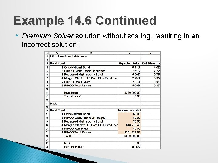
Example 14. 6 Continued Premium Solver solution without scaling, resulting in an incorrect solution!

Example 14. 6 Continued Solver solution after scaling the variables

Transportation Models The transportation problem involves determining how much to ship from a set of sources of supply (factories, warehouses, etc. ) to a set of demand locations (warehouses, customers, etc. ) at minimum cost.

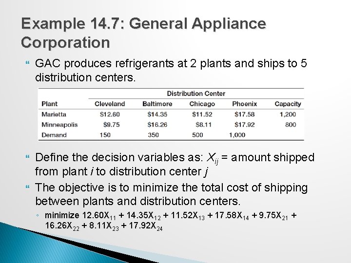
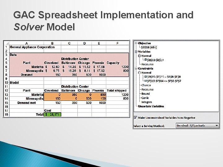
Example 14. 7: General Appliance Corporation GAC produces refrigerants at 2 plants and ships to 5 distribution centers. Define the decision variables as: Xij = amount shipped from plant i to distribution center j The objective is to minimize the total cost of shipping between plants and distribution centers. ◦ minimize 12. 60 X 11 + 14. 35 X 12 + 11. 52 X 13 + 17. 58 X 14 + 9. 75 X 21 + 16. 26 X 22 + 8. 11 X 23 + 17. 92 X 24

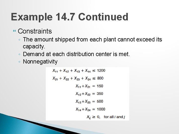
Example 14. 7 Continued Constraints ◦ The amount shipped from each plant cannot exceed its capacity. ◦ Demand at each distribution center is met. ◦ Nonnegativity

GAC Spreadsheet Implementation and Solver Model

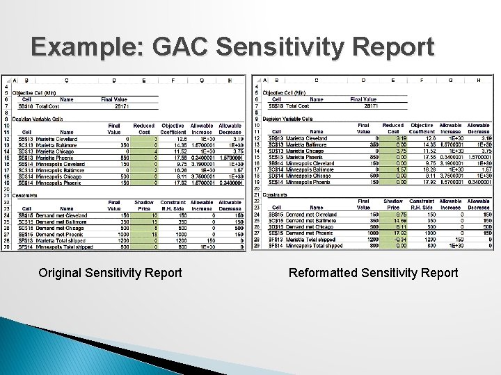
Formatting the Sensitivity Report Depending on how cells in your spreadsheet model are formatted, the Sensitivity report produced by Solver may not reflect the accurate values of reduced costs or shadow prices because an insufficient number of decimal places may be displayed. We highly recommend that after you save the Sensitivity report to your workbook, you select the reduced cost and shadow price ranges and format them to have at least two or three decimal places.

Example: GAC Sensitivity Report Original Sensitivity Report Reformatted Sensitivity Report

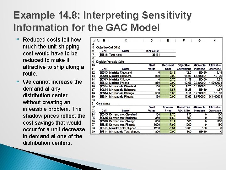
Example 14. 8: Interpreting Sensitivity Information for the GAC Model Reduced costs tell how much the unit shipping cost would have to be reduced to make it attractive to ship along a route. We cannot increase the demand at any distribution center without creating an infeasible problem. The shadow prices reflect the cost savings that would occur for a unit decrease in demand at one of the distribution centers.

Degeneracy The GAC solution exhibits a phenomenon called degeneracy. A solution is degenerate if the right-handside value of any constraint has a zero Allowable Increase or Allowable Decrease. ◦ Degeneracy can impact the interpretation of sensitivity analysis information. For example, reduced costs and shadow prices may not be unique, and you may have to change objective function coefficients beyond their allowable increases or decreases before the optimal solution will change.

Multiperiod Production Planning Models The basic decisions are how much to produce in each time period to meet anticipated demand over each period. Although it might seem obvious to simply produce to the anticipated level of sales, it may be advantageous to produce more than needed in earlier time periods when production costs may be lower and store the excess production as inventory for use in later time periods, thereby letting lower production costs offset the costs of holding the inventory.

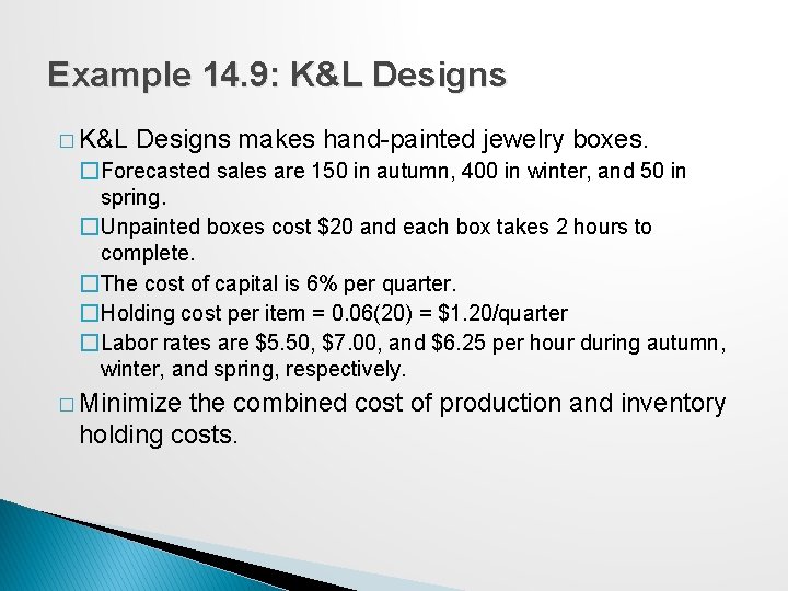
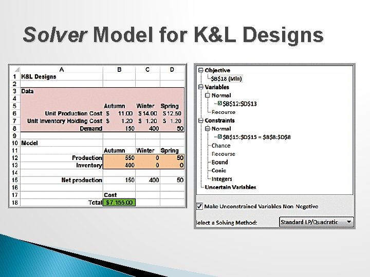
Example 14. 9: K&L Designs � K&L Designs makes hand-painted jewelry boxes. �Forecasted sales are 150 in autumn, 400 in winter, and 50 in spring. �Unpainted boxes cost $20 and each box takes 2 hours to complete. �The cost of capital is 6% per quarter. �Holding cost per item = 0. 06(20) = $1. 20/quarter �Labor rates are $5. 50, $7. 00, and $6. 25 per hour during autumn, winter, and spring, respectively. � Minimize the combined cost of production and inventory holding costs.

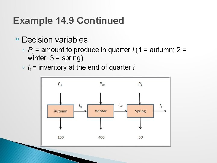
Example 14. 9 Continued Decision variables ◦ Pi = amount to produce in quarter i (1 = autumn; 2 = winter; 3 = spring) ◦ Ii = inventory at the end of quarter i

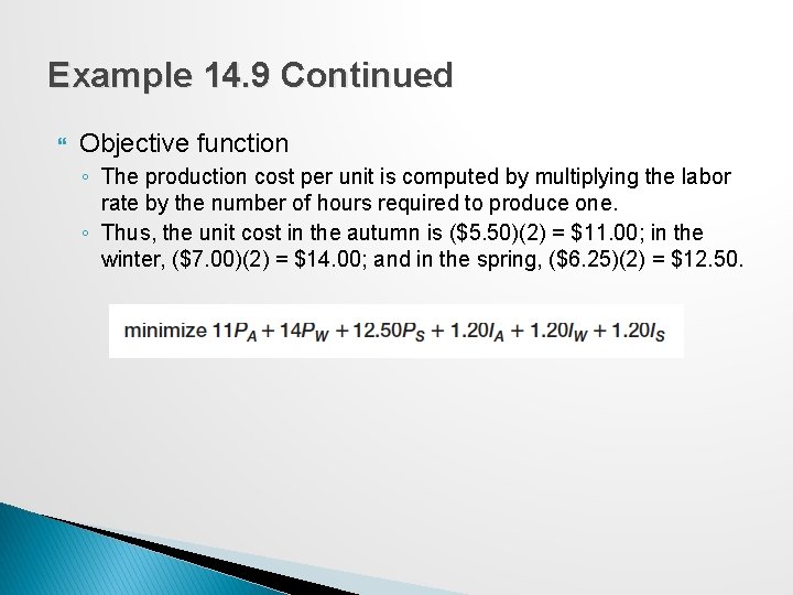
Example 14. 9 Continued Objective function ◦ The production cost per unit is computed by multiplying the labor rate by the number of hours required to produce one. ◦ Thus, the unit cost in the autumn is ($5. 50)(2) = $11. 00; in the winter, ($7. 00)(2) = $14. 00; and in the spring, ($6. 25)(2) = $12. 50.

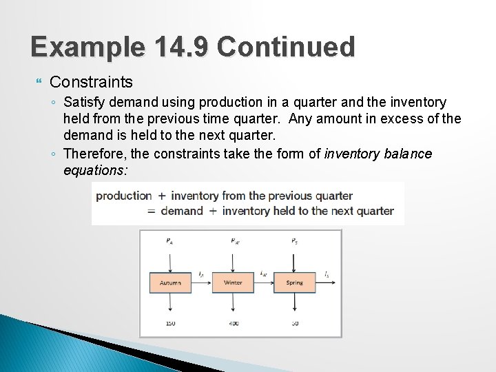
Example 14. 9 Continued Constraints ◦ Satisfy demand using production in a quarter and the inventory held from the previous time quarter. Any amount in excess of the demand is held to the next quarter. ◦ Therefore, the constraints take the form of inventory balance equations:

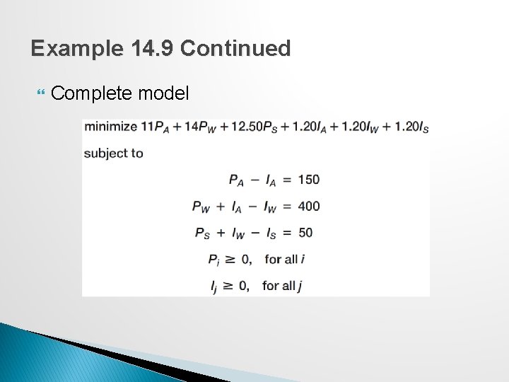
Example 14. 9 Continued Complete model

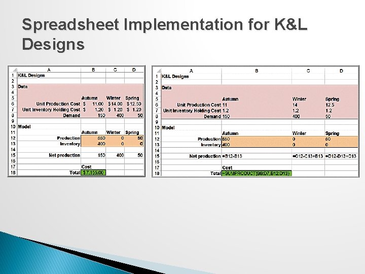
Spreadsheet Implementation for K&L Designs

Solver Model for K&L Designs

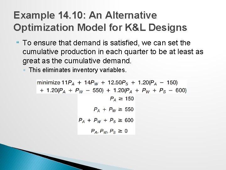
Example 14. 10: An Alternative Optimization Model for K&L Designs To ensure that demand is satisfied, we can set the cumulative production in each quarter to be at least as great as the cumulative demand. ◦ This eliminates inventory variables.

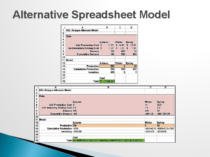
Alternative Spreadsheet Model

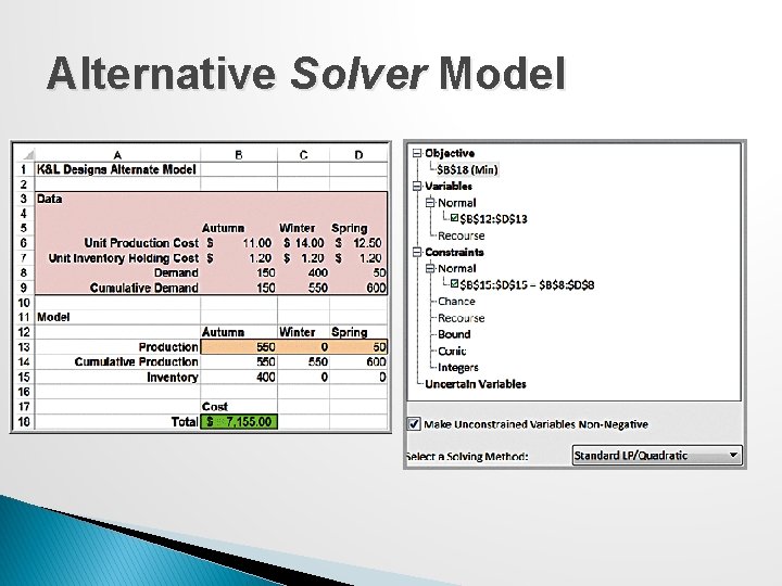
Alternative Solver Model

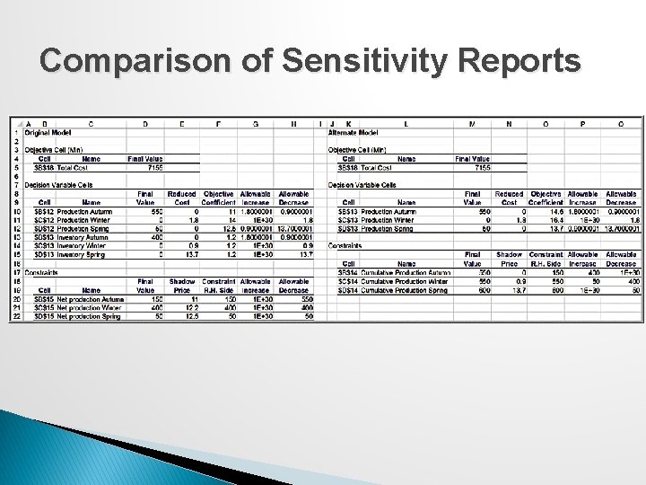
Comparison of Sensitivity Reports

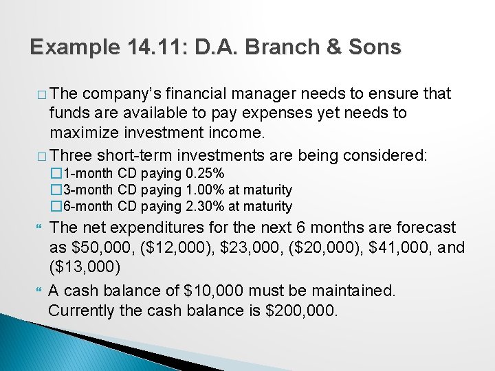
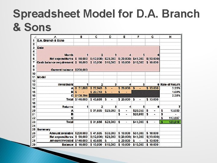
Example 14. 11: D. A. Branch & Sons � The company’s financial manager needs to ensure that funds are available to pay expenses yet needs to maximize investment income. � Three short-term investments are being considered: � 1 -month CD paying 0. 25% � 3 -month CD paying 1. 00% at maturity � 6 -month CD paying 2. 30% at maturity The net expenditures for the next 6 months are forecast as $50, 000, ($12, 000), $23, 000, ($20, 000), $41, 000, and ($13, 000) A cash balance of $10, 000 must be maintained. Currently the cash balance is $200, 000.

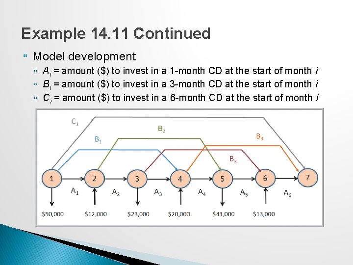
Example 14. 11 Continued Model development ◦ Ai = amount ($) to invest in a 1 -month CD at the start of month i ◦ Bi = amount ($) to invest in a 3 -month CD at the start of month i ◦ Ci = amount ($) to invest in a 6 -month CD at the start of month i

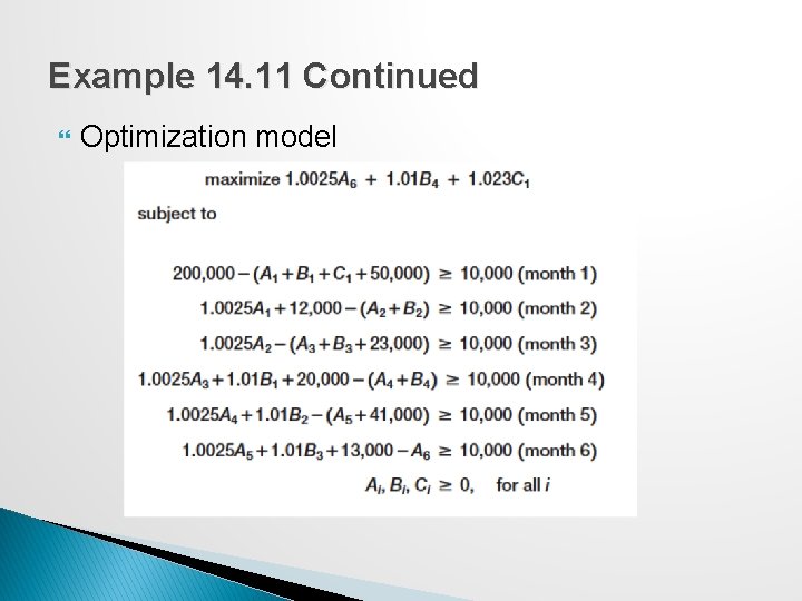
Example 14. 11 Continued Optimization model

Spreadsheet Model for D. A. Branch & Sons

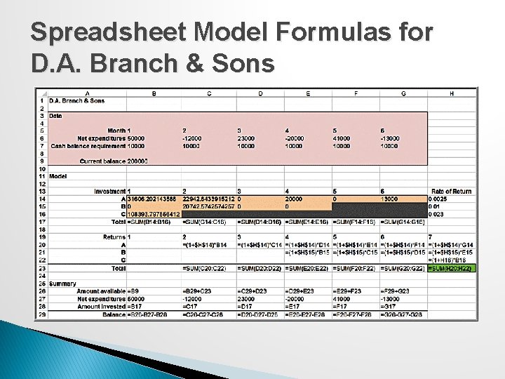
Spreadsheet Model Formulas for D. A. Branch & Sons

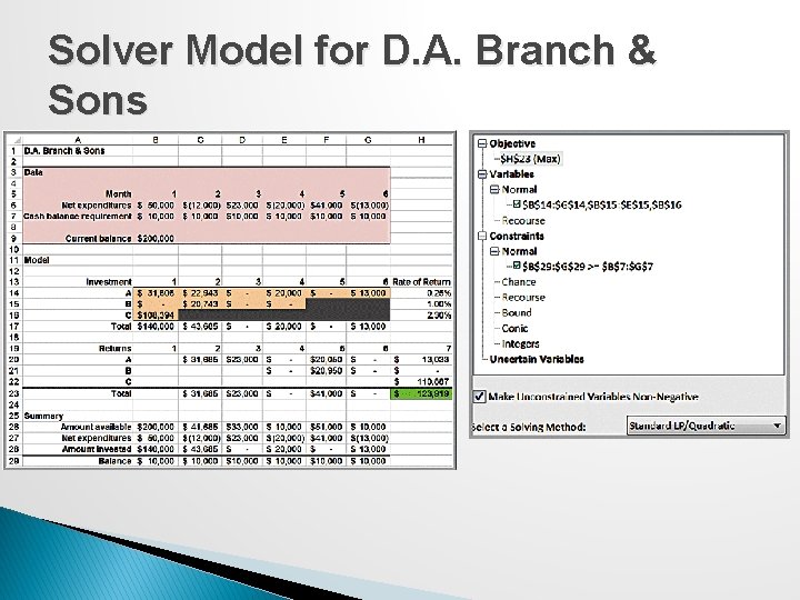
Solver Model for D. A. Branch & Sons

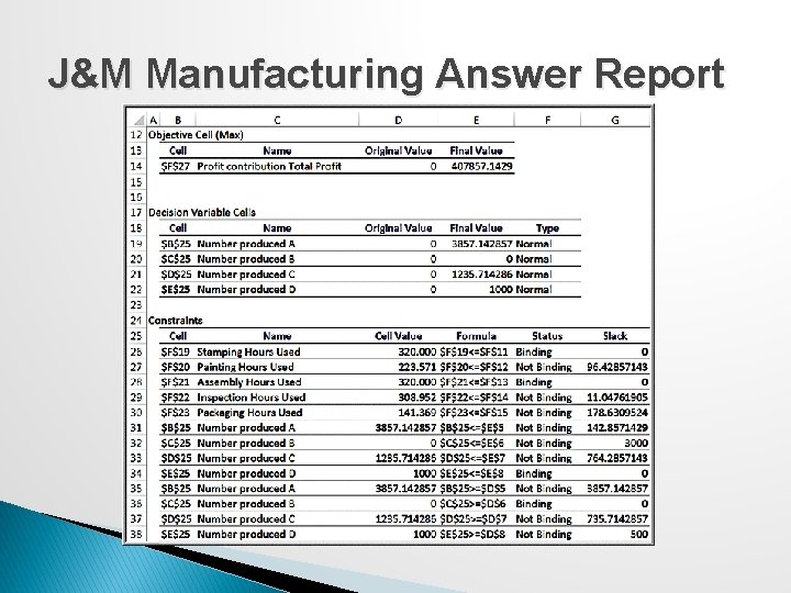
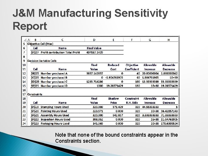
Models with Bounded Variables Solver handles simple lower bounds (e. g. , C ≥ 500) and upper bounds (e. g. , D ≤ 1, 000) quite differently from ordinary constraints in the Sensitivity report. Lower and upper bounds are treated in a manner similar to nonnegativity constraints, which also do not appear explicitly as constraints in the model. This makes it more difficult to interpret the sensitivity information, because we no longer have the shadow prices and allowable increases and decreases associated with these constraints.

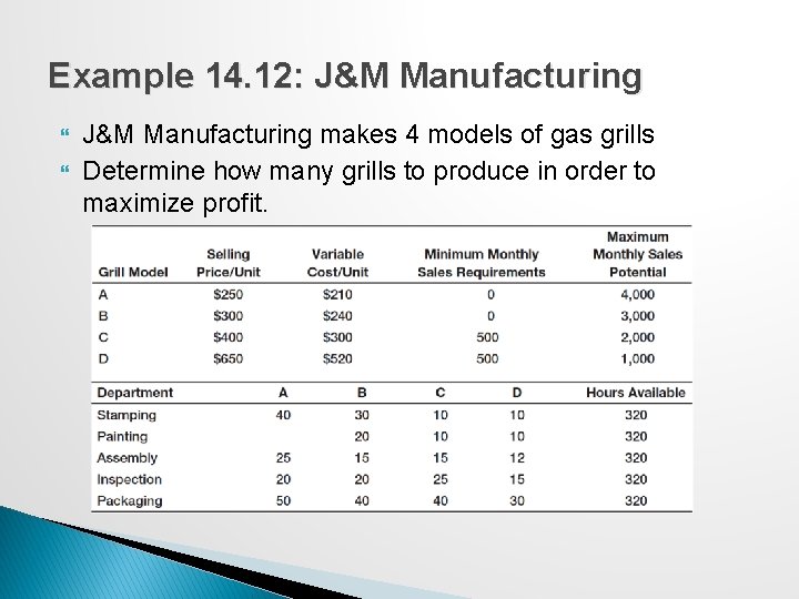
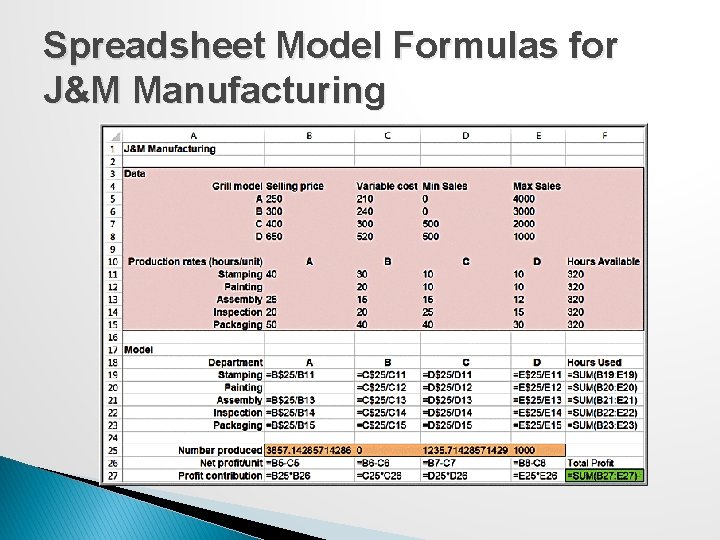
Example 14. 12: J&M Manufacturing makes 4 models of gas grills Determine how many grills to produce in order to maximize profit.

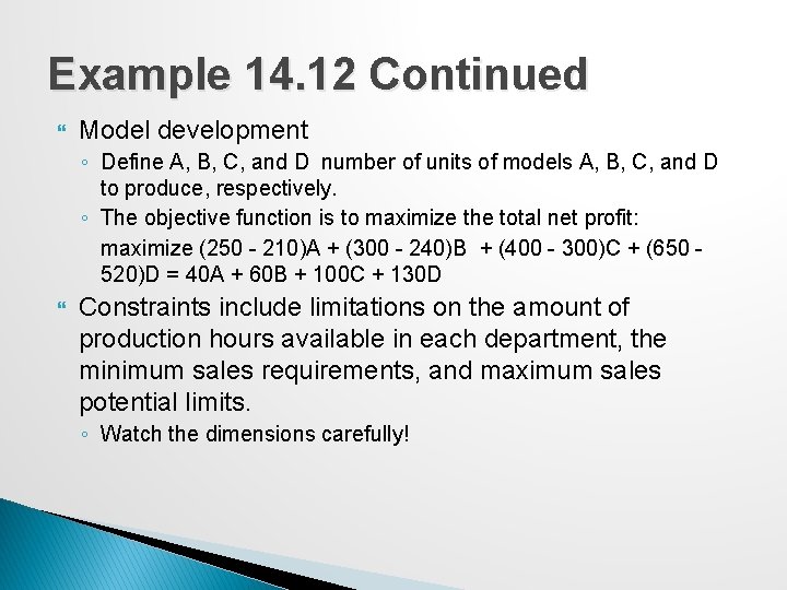
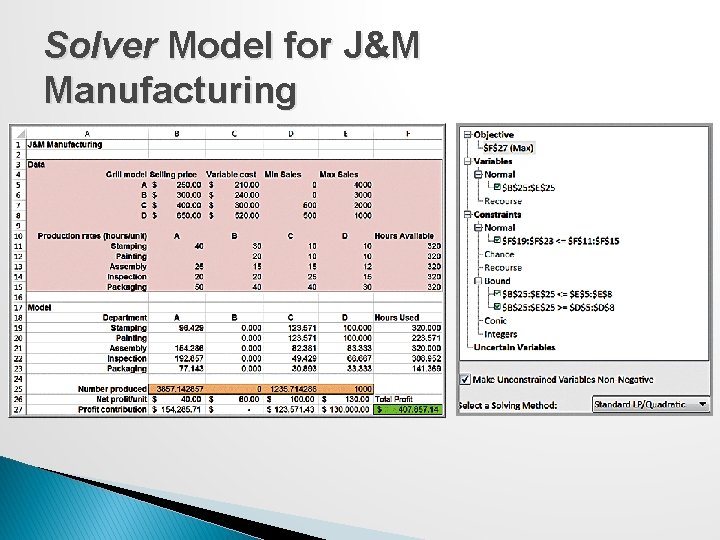
Example 14. 12 Continued Model development ◦ Define A, B, C, and D number of units of models A, B, C, and D to produce, respectively. ◦ The objective function is to maximize the total net profit: maximize (250 - 210)A + (300 - 240)B + (400 - 300)C + (650 520)D = 40 A + 60 B + 100 C + 130 D Constraints include limitations on the amount of production hours available in each department, the minimum sales requirements, and maximum sales potential limits. ◦ Watch the dimensions carefully!

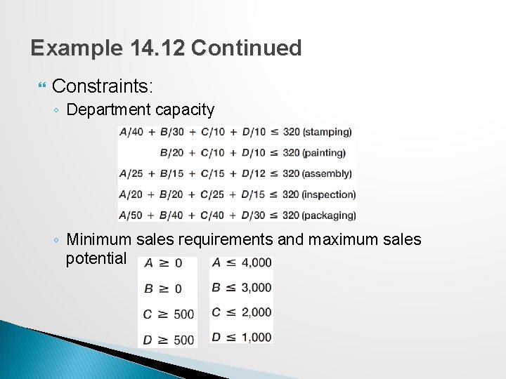
Example 14. 12 Continued Constraints: ◦ Department capacity ◦ Minimum sales requirements and maximum sales potential

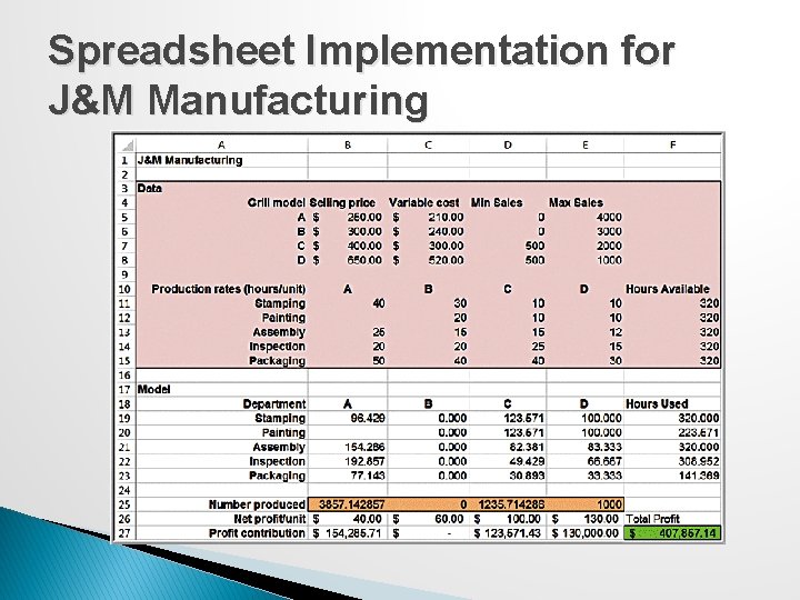
Spreadsheet Implementation for J&M Manufacturing

Spreadsheet Model Formulas for J&M Manufacturing

Solver Model for J&M Manufacturing

J&M Manufacturing Answer Report

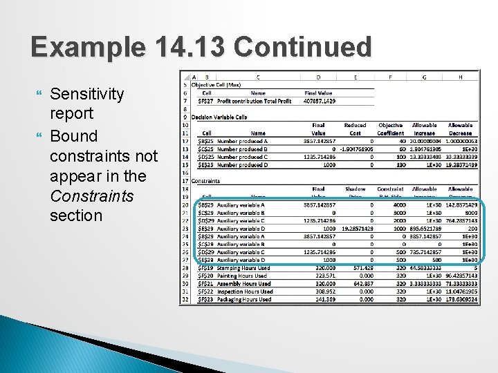
J&M Manufacturing Sensitivity Report Note that none of the bound constraints appear in the Constraints section.

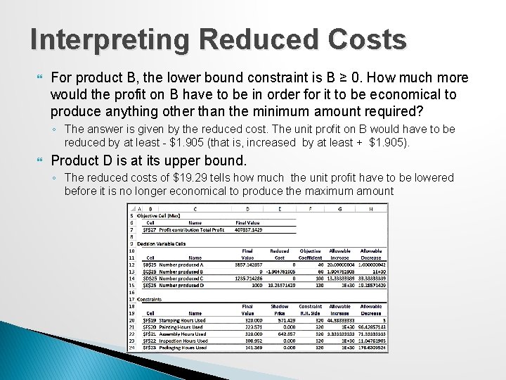
Interpreting Reduced Costs For product B, the lower bound constraint is B ≥ 0. How much more would the profit on B have to be in order for it to be economical to produce anything other than the minimum amount required? ◦ The answer is given by the reduced cost. The unit profit on B would have to be reduced by at least - $1. 905 (that is, increased by at least + $1. 905). Product D is at its upper bound. ◦ The reduced costs of $19. 29 tells how much the unit profit have to be lowered before it is no longer economical to produce the maximum amount

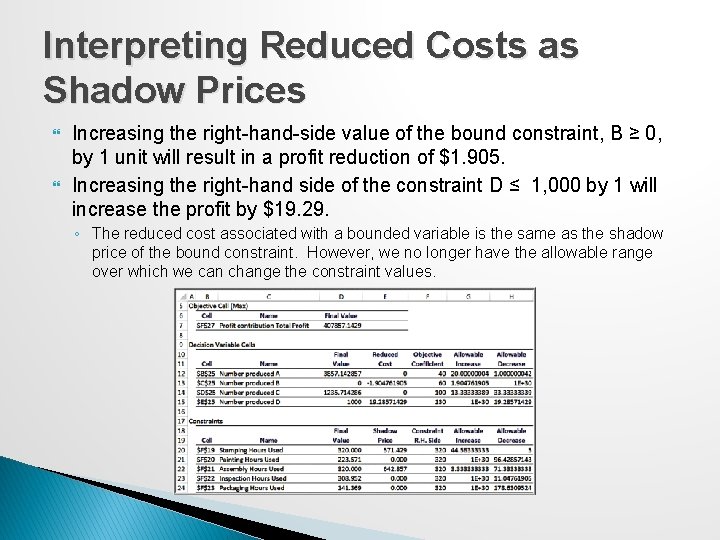
Interpreting Reduced Costs as Shadow Prices Increasing the right-hand-side value of the bound constraint, B ≥ 0, by 1 unit will result in a profit reduction of $1. 905. Increasing the right-hand side of the constraint D ≤ 1, 000 by 1 will increase the profit by $19. 29. ◦ The reduced cost associated with a bounded variable is the same as the shadow price of the bound constraint. However, we no longer have the allowable range over which we can change the constraint values.

Auxiliary Variables for Bound Constraints � Auxiliary variables are a new set of cells for any decision variables that have upper- or lower-bound constraints created by referencing (not copying) the original changing cells. �In the Solver model, use auxiliary variable cells—not the changing variable cells as defined—to define the bound constraints. �Auxiliary variables allow easier interpretation of shadow prices for bounded variables.

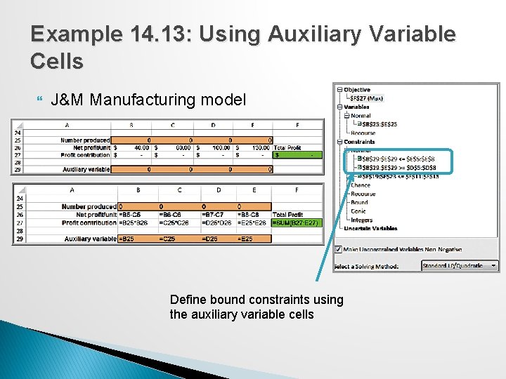
Example 14. 13: Using Auxiliary Variable Cells J&M Manufacturing model Define bound constraints using the auxiliary variable cells

Example 14. 13 Continued Sensitivity report Bound constraints not appear in the Constraints section

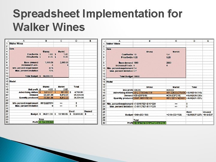
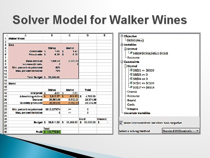
Example 14. 14: Walker Wines A production/marketing allocation problem � Walker Wines buys grapes from local growers and blends the pressings to make two types of wine (Shiraz and Merlot). Grape costs are $1. 60 per bottle Shiraz and $1. 40 per bottle Merlot. � Their contract requires between 40% and 70% of their wine to be Shiraz. Predicted demand for Shiraz is 1000 bottles but increases by 5 bottles for each dollar spent on advertising; the base demand for merlot is 2, 000 bottles and increases by 8 bottles for each $1 spent on advertising. Production should not exceed demand. Shiraz sells to retail stores for $6. 25 per bottle and merlot is sold for $5. 25 per bottle. $50, 000 is available to purchase grapes and advertise products.

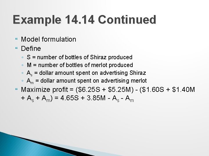
Example 14. 14 Continued Model formulation Define ◦ ◦ S = number of bottles of Shiraz produced M = number of bottles of merlot produced As = dollar amount spent on advertising Shiraz Am = dollar amount spent on advertising merlot Maximize profit = ($6. 25 S + $5. 25 M) - ($1. 60 S + $1. 40 M + As + Am) = 4. 65 S + 3. 85 M - As - Am

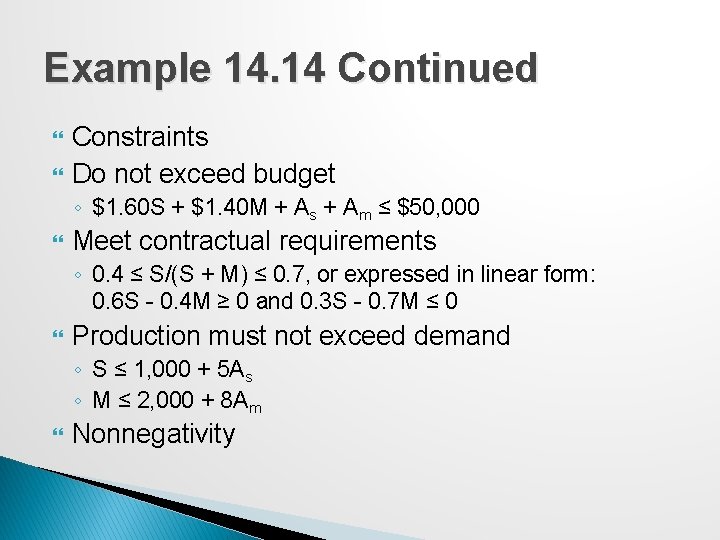
Example 14. 14 Continued Constraints Do not exceed budget ◦ $1. 60 S + $1. 40 M + As + Am ≤ $50, 000 Meet contractual requirements ◦ 0. 4 ≤ S/(S + M) ≤ 0. 7, or expressed in linear form: 0. 6 S - 0. 4 M ≥ 0 and 0. 3 S - 0. 7 M ≤ 0 Production must not exceed demand ◦ S ≤ 1, 000 + 5 As ◦ M ≤ 2, 000 + 8 Am Nonnegativity

Spreadsheet Implementation for Walker Wines

Solver Model for Walker Wines

Using Sensitivity Information Correctly One crucial assumption in interpreting sensitivity analysis information for changes in model parameters is that all other model parameters are held constant.

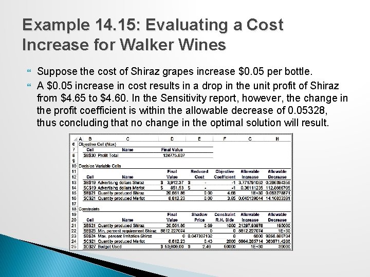
Example 14. 15: Evaluating a Cost Increase for Walker Wines Suppose the cost of Shiraz grapes increase $0. 05 per bottle. A $0. 05 increase in cost results in a drop in the unit profit of Shiraz from $4. 65 to $4. 60. In the Sensitivity report, however, the change in the profit coefficient is within the allowable decrease of 0. 05328, thus concluding that no change in the optimal solution will result.

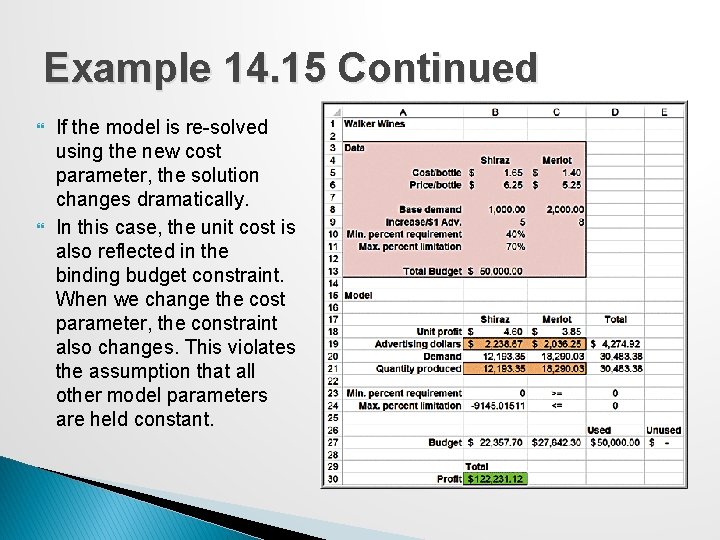
Example 14. 15 Continued If the model is re-solved using the new cost parameter, the solution changes dramatically. In this case, the unit cost is also reflected in the binding budget constraint. When we change the cost parameter, the constraint also changes. This violates the assumption that all other model parameters are held constant.