Nonlinear OpAmp Circuits Most typical applications require op

Nonlinear Op-Amp Circuits • Most typical applications require op amp and its components to act linearly – I-V characteristics of passive devices such as resistors, capacitors should be described by linear equation (Ohm’s Law) – For op amp, linear operation means input and output voltages are related by a constant proportionality (Av should be constant) • Some application require op amps to behave in nonlinear manner (logarithmic and antilogarithmic amplifiers) Visit for more Learning Resources

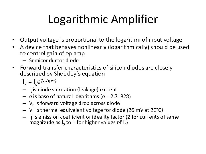
Logarithmic Amplifier • Output voltage is proportional to the logarithm of input voltage • A device that behaves nonlinearly (logarithmically) should be used to control gain of op amp – Semiconductor diode • Forward transfer characteristics of silicon diodes are closely described by Shockley’s equation IF = Ise(VF/ηVT) – – – Is is diode saturation (leakage) current e is base of natural logarithms (e = 2. 71828) VF is forward voltage drop across diode VT is thermal equivalent voltage for diode (26 m. V at 20°C) η is emission coefficient or ideality factor (2 for currents of same magnitude as IS to 1 for higher values of IF)

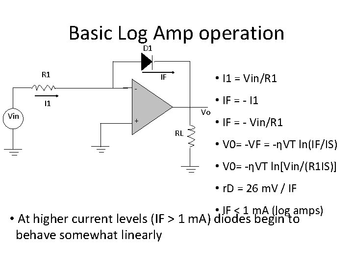
Basic Log Amp operation D 1 R 1 • I 1 = Vin/R 1 IF - I 1 Vin Vo + RL • IF = - I 1 • IF = - Vin/R 1 • V 0= -VF = -ηVT ln(IF/IS) • V 0= -ηVT ln[Vin/(R 1 IS)] • r. D = 26 m. V / IF • IF < 1 m. A (log amps) • At higher current levels (IF > 1 m. A) diodes begin to behave somewhat linearly

Logarithmic Amplifier • Linear graph: voltage gain is very high for low input voltages and very low for high input voltages • Semilogarithmic graph: straight line proves logarithmic nature of amplifier’s transfer characteristic • Transfer characteristics of log amps are usually expressed in terms of slope of V 0 versus Vin plot in milivolts per decode • η affects slope of transfer curve; IS determines the y intercept Operational Amplifiers and Linear Integrated Circuits: Theory and Applications by Denton J. Dailey

Additional Log Amp Variations Q 1 R 1 IC IE - Vo = VBE I 1 Vin + RL IC = IESe (VBE/VT) - IES is emitter saturation current - VBE is drop across base-emitter junction • Often a transistor is used as logging element in log amp (transdiode configuration) • Transistor logging elements allow operation of log amp over wider current ranges (greater dynamic range)

Antilogarithmic Amplifier • Output of an antilog amp is proportional to the antilog of the input voltage • with diode logging element – V 0 = -RFISe(Vin/VT) • With transdiode logging element – V 0 = -RFIESe(Vin/VT) • As with log amp, it is necessary to know saturation currents and to tightly control junction temperature

Antilogarithmic Amplifier RF IE Q 1 Vin R 1 Vin I 1 + (α = 1) I 1 = IC = IE IF D 1 I 1 Vo + RL IF Vo RL

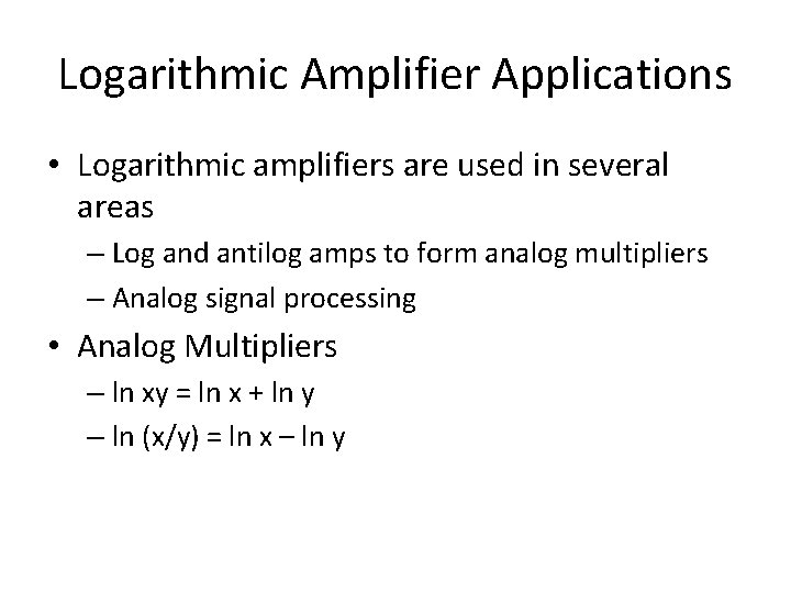
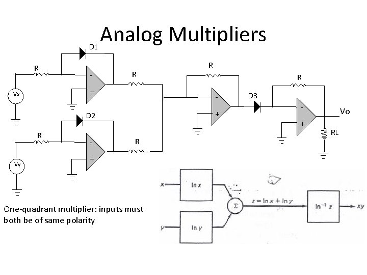
Logarithmic Amplifier Applications • Logarithmic amplifiers are used in several areas – Log and antilog amps to form analog multipliers – Analog signal processing • Analog Multipliers – ln xy = ln x + ln y – ln (x/y) = ln x – ln y

D 1 R - Analog Multipliers R + Vx Vy - R + D 2 R R R + One-quadrant multiplier: inputs must both be of same polarity Operational Amplifiers and Linear Integrated Circuits: Theory and Applications by Denton J. Dailey D 3 + Vo RL

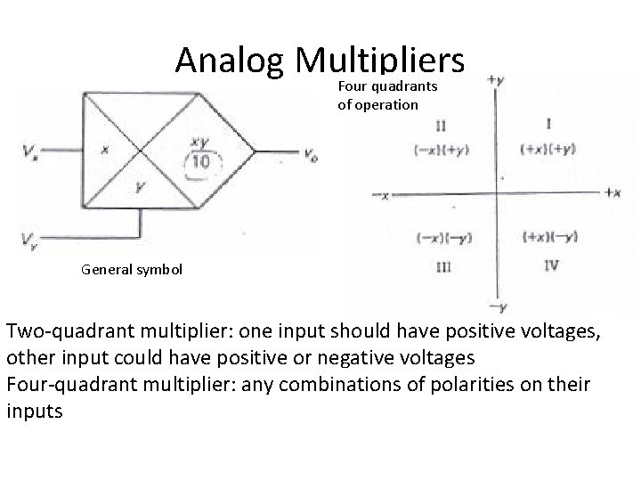
Analog Multipliers Four quadrants of operation General symbol Two-quadrant multiplier: one input should have positive voltages, other input could have positive or negative voltages Four-quadrant multiplier: any combinations of polarities on their inputs Operational Amplifiers and Linear Integrated Circuits: Theory and Applications by Denton J. Dailey

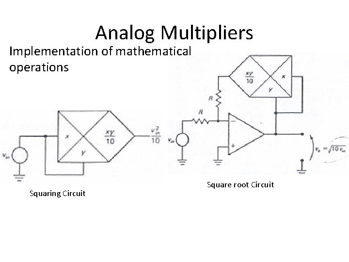
Analog Multipliers Implementation of mathematical operations Square root Circuit Squaring Circuit Operational Amplifiers and Linear Integrated Circuits: Theory and Applications by Denton J. Dailey

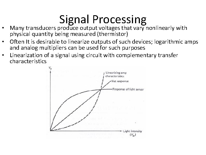
Signal Processing • Many transducers produce output voltages that vary nonlinearly with physical quantity being measured (thermistor) • Often It is desirable to linearize outputs of such devices; logarithmic amps and analog multipliers can be used for such purposes • Linearization of a signal using circuit with complementary transfer characteristics

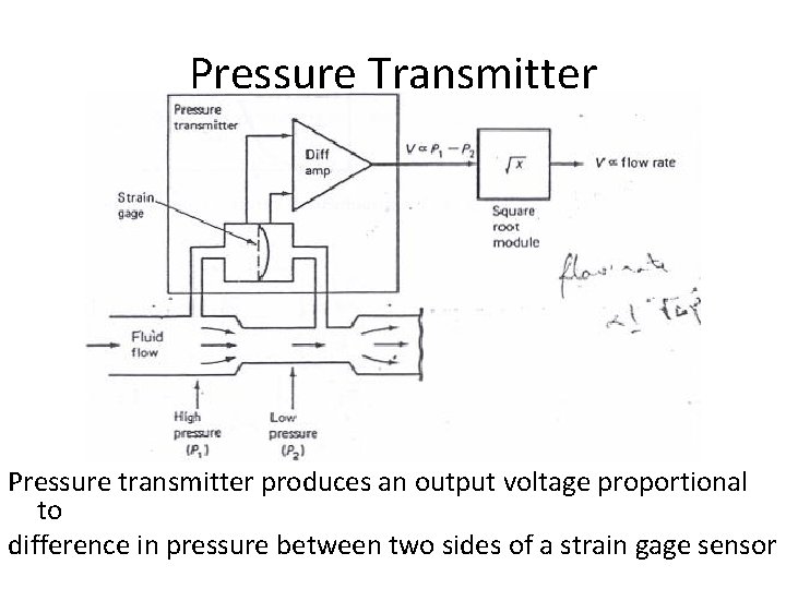
Pressure Transmitter Pressure transmitter produces an output voltage proportional to difference in pressure between two sides of a strain gage sensor Operational Amplifiers and Linear Integrated Circuits: Theory and Applications by Denton J. Dailey

Pressure Transmitter • A venturi is used to create pressure differential across strain gage • Output of transmitter is proportional to pressure differential • Fluid flow through pipe is proportional to square root of pressure differential detected by strain gage • If output of transmitter is processed through a square root amplifier, an output directly proportional to flow rate is obtained

Precision Rectifiers • Op amps can be used to form nearly ideal rectifiers (convert ac to dc) • Idea is to use negative feedback to make op amp behave like a rectifier with near-zero barrier potential and with linear I/O characteristic • Transconductance curves for typical silicon diode and an ideal diode

Precision Half-Wave. RF Rectifier D 1 R 1 I 2 Vin D 2 I 1 Vo + I 2 Vx RL • Solid arrows represent current flow for positive half-cycles of Vin and dashed arrows represent current flow for negative half-cycles

Precision Half-Wave Rectifier • If signal source is going positive, output of op amp begins to go negative, forward biasing D 1 – Since D 1 is forward biased, output of op amp Vx will reach a maximum level of ~ 0. 7 V regardless of how far positive Vin goes – This is insufficient to appreciably forward bias D 2, and V 0 remains at 0 V • On negative-going half-cycles, D 1 is reverse-biased and D 2 is forward biased – Negative feedback reduces barrier potential of D 2 to 0. 7 V/AOL (~ = 0) – Gain of circuit to negative-going portions of Vin is given by AV = -RF/R 1 Operational Amplifiers and Linear Integrated Circuits: Theory and Applications by Denton J. Dailey

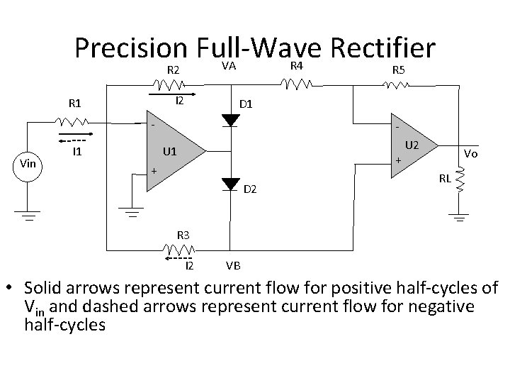
Precision Full-Wave Rectifier VA R 4 R 5 R 2 I 2 R 1 D 1 Vin U 1 I 1 + + D 2 U 2 Vo RL R 3 I 2 VB • Solid arrows represent current flow for positive half-cycles of Vin and dashed arrows represent current flow for negative half-cycles

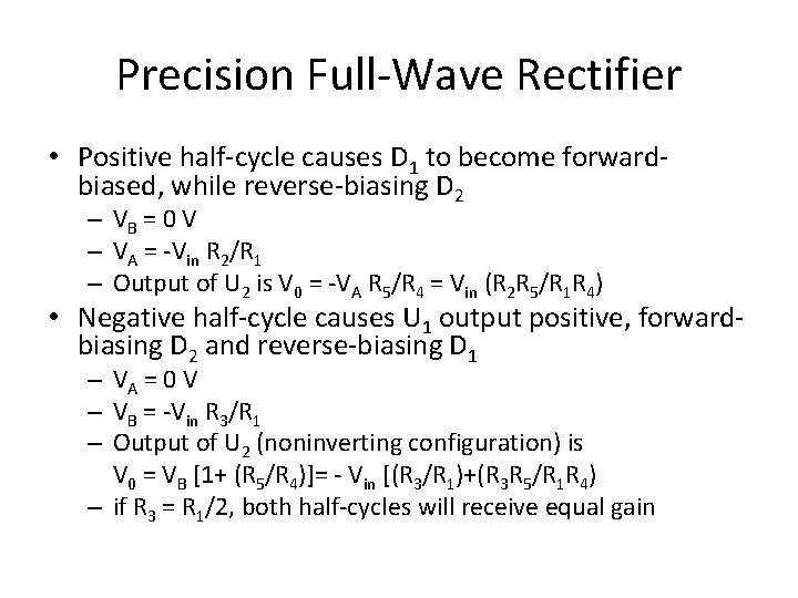
Precision Full-Wave Rectifier • Positive half-cycle causes D 1 to become forwardbiased, while reverse-biasing D 2 – VB = 0 V – VA = -Vin R 2/R 1 – Output of U 2 is V 0 = -VA R 5/R 4 = Vin (R 2 R 5/R 1 R 4) • Negative half-cycle causes U 1 output positive, forwardbiasing D 2 and reverse-biasing D 1 – VA = 0 V – VB = -Vin R 3/R 1 – Output of U 2 (noninverting configuration) is V 0 = VB [1+ (R 5/R 4)]= - Vin [(R 3/R 1)+(R 3 R 5/R 1 R 4) – if R 3 = R 1/2, both half-cycles will receive equal gain

Precision Rectifiers • Useful when signal to be rectified is very low in amplitude and where good linearity is needed • Frequency and power handling limitations of op amps limit the use of precision rectifiers to low-power applications (few hundred k. Hz) • Precision full-wave rectifier is often referred to as absolute magnitude circuit

ACTIVE FILTERS

Active Filters • Op amps have wide applications in design of active filters • Filter is a circuit designed to pass frequencies within a specific range, while rejecting all frequencies that fall outside this range • Another class of filters are designed to produce an output that is delayed in time or shifted in phase with respect to filter’s input • Passive filters: constructed using only passive components (resistors, capacitors, inductors) • Active filters: characteristics are augmented using one or more amplifiers; constructed using op amps, resistors, and capacitors only – Allow many filter parameters to be adjusted continuously and at will

Filter Fundamentals • Five basic types of filters – Low-pass (LP) – High-pass (HP) – Bandpass (BP) – Bandstop (notch or band-reject) – All-pass (or time-delay)

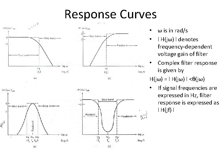
Response Curves • ω is in rad/s • l H(jω) l denotes frequency-dependent voltage gain of filter • Complex filter response is given by H(jω) = l H(jω) l <θ(jω) • If signal frequencies are expressed in Hz, filter response is expressed as l H(jf) l Operational Amplifiers and Linear Integrated Circuits: Theory and Applications by Denton J. Dailey

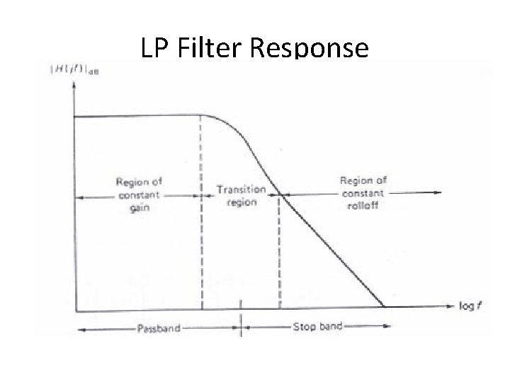
Filter Terminology • Filter passband: range of frequencies a filter will allow to pass, either amplified or relatively unattenuated • All other frequencies are considered to fall into filter’s stop band(s) • Frequency at which gain of filter drops by 3. 01 d. B from that of passband determines where stop band begins; this frequency is called corner frequency (fc) • Response of filter is down by 3 d. B at corner frequency (3 d. B decrease in voltage gain translates to a reduction of 50% in power delivered to load driven by filter) • fc is often called half-power point

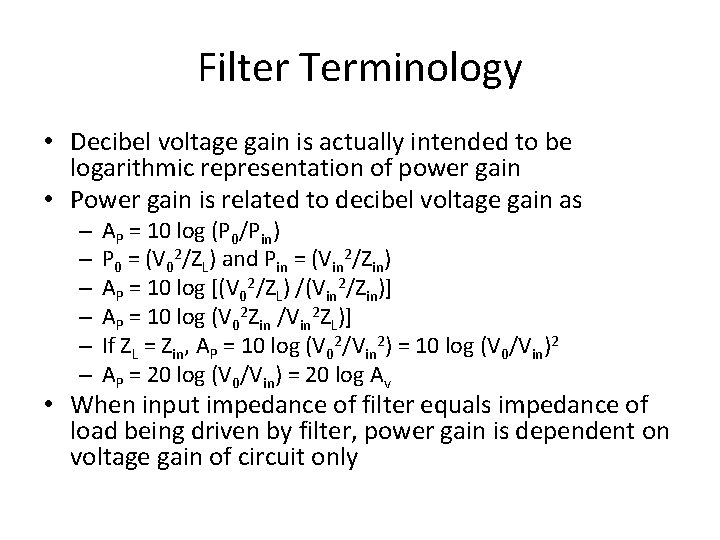
Filter Terminology • Decibel voltage gain is actually intended to be logarithmic representation of power gain • Power gain is related to decibel voltage gain as – – – AP = 10 log (P 0/Pin) P 0 = (V 02/ZL) and Pin = (Vin 2/Zin) AP = 10 log [(V 02/ZL) /(Vin 2/Zin)] AP = 10 log (V 02 Zin /Vin 2 ZL)] If ZL = Zin, AP = 10 log (V 02/Vin 2) = 10 log (V 0/Vin)2 AP = 20 log (V 0/Vin) = 20 log Av • When input impedance of filter equals impedance of load being driven by filter, power gain is dependent on voltage gain of circuit only

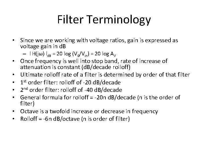
Filter Terminology • Since we are working with voltage ratios, gain is expressed as voltage gain in d. B – l H(jω) ld. B = 20 log (V 0/Vin) = 20 log AV • Once frequency is well into stop band, rate of increase of attenuation is constant (d. B/decade rolloff) • Ultimate rolloff rate of a filter is determined by order of that filter • 1 st order filter: rolloff of -20 d. B/decade • 2 nd order filter: rolloff of -40 d. B/decade • General formula for rolloff = -20 n d. B/decade (n is the order of filter) • Octave is a twofold increase or decrease in frequency • Rolloff = -6 n d. B/octave (n is order of filter)

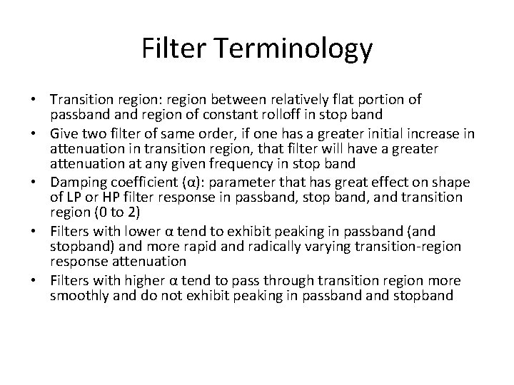
Filter Terminology • Transition region: region between relatively flat portion of passband region of constant rolloff in stop band • Give two filter of same order, if one has a greater initial increase in attenuation in transition region, that filter will have a greater attenuation at any given frequency in stop band • Damping coefficient (α): parameter that has great effect on shape of LP or HP filter response in passband, stop band, and transition region (0 to 2) • Filters with lower α tend to exhibit peaking in passband (and stopband) and more rapid and radically varying transition-region response attenuation • Filters with higher α tend to pass through transition region more smoothly and do not exhibit peaking in passband stopband

LP Filter Response Operational Amplifiers and Linear Integrated Circuits: Theory and Applications by Denton J. Dailey

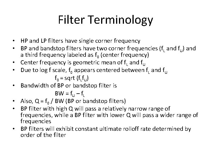
Filter Terminology • HP and LP filters have single corner frequency • BP and bandstop filters have two corner frequencies (f. L and f. U) and a third frequency labeled as f 0 (center frequency) • Center frequency is geometric mean of f. L and f. U • Due to log f scale, f 0 appears centered between f. L and f. U f 0 = sqrt (f. Lf. U) • Bandwidth of BP or bandstop filter is BW = f. U – f. L • Also, Q = f 0 / BW (BP or bandstop filters) • BP filter with high Q will pass a relatively narrow range of frequencies, while a BP filter with lower Q will pass a wider range of frequencies • BP filters will exhibit constant ultimate rolloff rate determined by order of the filter

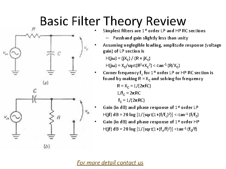
Basic Filter Theory Review • • • Simplest filters are 1 st order LP and HP RC sections – Passband gain slightly less than unity Assuming neglegible loading, amplitude response (voltage gain) of LP section is H(jω) = (j. XC) / (R + j. XC) H(jω) = XC/sqrt(R 2+XC 2) <-tan-1 (R/XC) Corner frequency fc for 1 st order LP or HP RC section is found by making R = XC and solving for frequency R = XC = 1/(2πf. C) 1/f. C = 2πRC f. C = 1/(2πRC) Gain (in d. B) and phase response of 1 st order LP H(jf) d. B = 20 log [1/{sqrt(1+(f/fc)2}] <-tan-1 (f/f. C) Gain (in d. B) and phase response of 1 st order HP H(jf) d. B = 20 log [1/{sqrt(1+(fc/f)2}] <tan-1 (f. C/f) For more detail contact us Operational Amplifiers and Linear Integrated Circuits: Theory and Applications by Denton J. Dailey