DMOR Linear Programming Unconstrained optimization Constrained optimization Linear

DMOR Linear Programming

• Unconstrained optimization • Constrained optimization – Linear programming – Non-linear programming – arch. planning Constrained optimization elements: 1. decision variables 2. objective function 3. constraints 4. variable bounds

Bike company • Bike company produces: – Mountain bikes – Race bikes • Wants to maximize profit by setting quantities of each bike produced • No demand restrictions • Two teams produce two kinds of bikes: – Mountain bike team can produce up to 2 bikes per day – Race bike team can produce up to 3 bikes per day • Equal amount of time using metal finishing machine is needed for both kinds of bikes. – Up to 4 bikes can go through the machine daily • The acountant estimates profits for each bike – Mountain $15 – Race $10

Solution • Intuitive solution – We produce as many mountain bikes as possible (max 2) and what’s left goes for race bikes (2). – Generated Profit: $30+$20=$50. • Linear programming – Decision variables: Number of mountain x 1 and race x 2 bikes – Nonnegative: x 1≥ 0, x 2≥ 0 – Objective function: max daily profit: max Z=15 x 1+10 x 2 (in $/day) – Constraints: • Daily mountain bike production limit: x 1≤ 2 (in bikes/day) • Daily race bike production limit: x 2≤ 3 (in bikes/day) • Metal finishing machine limit: x 1+x 2 ≤ 4 (in bikes/day)

Corners are important • feasible region • Isoprofit lines are parallel • Profit increases the most for the gradient direction • Corners stick outside the most • Optimum is a corner or a an edge together with two endpoint (neighbouring) corners • If two corners are optimal then the line between them is also

Linear programming assumptions • Linear in decision variables – Additivity and proportionality • Excludes curves, step-functions, interaction factors, e. g. 5 x 1 x 2, start-up costs – Decision variables are real-valued • And not integer-valued • Programming in general assumes knowledge of all the parameters – Nevertheless we can do sensitivity analysis

An LP problem in standard form Features: • Objective is to maximze • Constraints only ≤ • Non-negative constraints’ RHS • Decision variables are nonnegative Algebraic formulation: • Objective function: • m functional constraints: • Variable bounds

Definitions • • solution cornerpoint solution feasible cornerpoint solution adjacent cornerpoint solutions

Key properties 1. Optimal cornerpoint solution is always a feasible cornerpoint solution 2. If objective function value for a given feasible cornerpoint solution is not less than the objective function value for all feasible adjacent cornerpoint solution, then this solution is optimal 3. There is finite number of feasible cornerpoint solutions Implications 1. Search the cornerpoints 2. Easy to say which cornerpoint is optimal 3. Algorithm will stop after finite number of iterations

Simplex method Two phases: 1. Start-up – find any feasible cornerpoint solution – – 2. Standard form is good because the orgin is always a feasible cornerpoint solution If not in standard form, we need additional procedure (to be described later) Iterations – move to adjacent feasible cornerpoint solutions such that each time you improve the objective function value – Stop when no improvement possible

Algebraic method • Millions of decision variables in real applications • Graphical method not possible • Algebraic method works fine – Inequality constraints changed into equality constraints – Solving a system of equations being a subset of all constraints • Subset – since commonly not all equalities mey hold at the same time • We need a way to remember which equalities are in the subset (active constraints) • We introduce slack variables e. g. x 1 ≤ 2 changed into x 1 + s 1 = 2, where s 1 ≥ 0 is a slack variable

Bike company • Two dimensional problem becomes now five-dimesional – Slack variable is positive only if the corresponding constraint is active More concepts: • augmented solution: values given for all variables, e. g. extended optimal cornersolution for Bike company is x 1, x 2, s 1, s 2, s 3 = (2, 2, 0, 1, 0) • basic solution: extended cornerpoint solution (feasible or infeasible), e. g. (2, 3, 0, 0, -1) is basic infeasible solution • basic feasible solution: feasible cornerpoint solution e. g. (0, 3, 2, 0, 1)

Setting variable values • degrees of freedom df df = (number of variables) - (number of independent equalities) • Simplex method automatically assigns zero value (corresponding constraint active) to df out of all variables and then determines the other values – – – x 1=0 means that constraint x 1 ≥ 0 is active x 2=0 means that constraint x 2 ≥ 0 is active s 1=0 means that constraint x 1 ≤ 2 is active s 2=0 means that constraint x 2 ≤ 3 is active s 3=0 means that constraint x 1+x 2 ≤ 4 is active • In our example df=2, hence two variables will be assigned a zero value

• More terminology – nonbasic variable: variable which currently is assigned a zero value – basic variable: variable which is currently NOT assigned a zero value • In standard form positive • Zero in special cases – basis: the set of current basic variables MANTRA: Nonbasic, value zero, constraint active • We can guess the basis but we have to be careful – We can get infeasible cornerpoint solution (previous picture) – No cornerpoint at all (below)

Moving to a better adjacent feasible cornerpoint solution • Adjacent cornerpoint solution is a good choice because: – In two adjacent cornerpoints the basic and nonbasic set are identical but for one element – Example • Point A: nonbasic set = {s 2, s 3}, basic set = {x 1, x 2, s 1} • Point B: nonbasic set = {s 1, s 2}, basic set = {x 1, x 2, s 3} This is necessary yet not sufficient condition for adjacency (vide (0, 4) and (4, 0))

• Three conditions for moving to a new cornerpoint solution – Have to be adjacent – Have to be feasible – The new solution have to be better than the old one • Two steps: 1. 2. Determine a nonbasic variable which improves the objective function most. Move this variable into basic set (entering basic variable) Increase value of entering basic variable up to the moment one of the basic variables reaches zero. Move this variable into nonbasic set (leaving basic variable) • x 1 improves objective function most • Constraint x 1 ≥ 0 ceases to be active • Only x 1 increases so we know the movement direction • The constraint which will be crossed over first is x 1 ≤ 2.

Algebraically • In the origin the situation is the following: – Basic variables: s 1, s 2, s 3 – Nonbasic variables: x 1, x 2 – Basic entering variable: x 1 • In a new cornerpoint solution, which is located at the intersection of the edges of two constraints x 2 ≥ 0 and x 1 ≤ 2 (point (2, 0)), we have: – Basic variables: x 1, s 2, s 3 – Nonbasic variables: x 2, s 1 • We exchanged x 1 for s 1

Minimum ratio test • In order to find basci leaving variable we have to find the smallest value for the following ratio: • In our example, the denominator is always 1. Generally it doesn’t have to be that way. • Two special cases: – Entering basic variable coefficient is 0 (the constraints do not intersect) – Entering basic variable coefficient is negative (the constraints intersect but the entering basic variable increases in the opposite direction in relation to the intersection point)

Finding a new basic feasible solution • We found a new basis – what then? • We can suibstitute zero into all nonbasic variables and solve the resulting system of m x m equations by Gaussian elimination • More effective is to perform only a part of Gaussian elimination in each step • When to stop iterating? (Joke about a computer scientist) – When we cannot find basic entering variable

Simplex method

Simplex tableau • Starting point • Tableau in proper form – One basic variable for each equality – Basic variable coefficient always +1 and coefficients above and below are zero – Z is treated as a basic variable of the objective function • The advantage of the proper form is taht we cann read current solution directly from the tableau.

2. 1 Are we done? No, we have 2 negative coefficients in the first raw 2. 2 Choose basic entering variable Most negative coefficient is for x 1 2. 3 Choose basic leaving variable Minimal ratio test: • If there is 0 or negative number in the pivot column write „no limit” • The smallest value is 2: the corresponding raw is called the pivot raw Pivot element

2. 4 Update the tableau a) In „basic variable” column exchange basic leaving variable with basic entering variable b) If pivot element is not equal to 1, divide all pivot raw coefficients by pivot element value c) But for the pivot element, we make all the coefficients in the pivot column equal to zero

Continued • New solution (x 1, x 2, s 1, s 2, s 3)=(2, 0, 0, 3, 2), Objective function value Z=30 2. 1 We are not optimal yet 2. 2, 2. 3 A new basic entering and leaving variable 2. 4 Back to proper form

Special cases • A draw when choosing basic entering variable, e. g. Z = 15 x 1+15 x 2 • A draw when choosing basic leaving variable – choose the one you want – the corner will the same anyway – A variable which was not chosen for the basic leaving variable will remain basic but will have a calculated value of 0 – A variable which was chosen will have an assigned value of 0 Basic feasible solution in such case is called degenerate and can lead to cycles in more than two dimensions (corners A, C – B, C – A, C)

• Minimal ratio test gives „no limit” everywhere – unbounded problem – no solution – Usually mean you forgot some constraint • In the optimal solution coefficients of some nonbasic variables have value of zero in the objective function raw – Choosing this variable to enter the basis has no effect on the objective function value – But it changes basic feasible solution – It means we have multiple optimum solutions

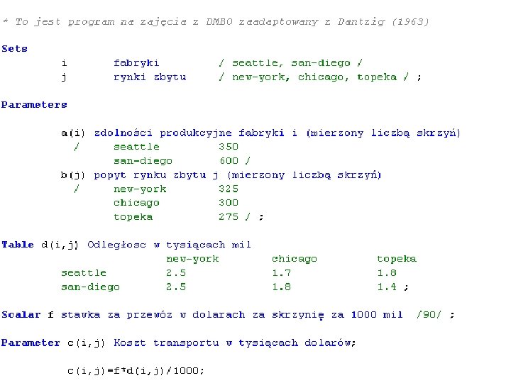
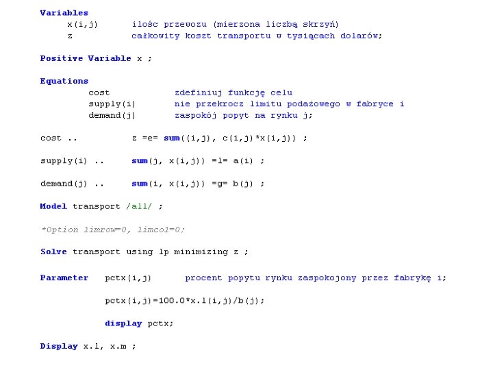
In practice • input formats: – Algebraic formulation – Spreadsheet formulation (columns: variables, raws: constraints) – Algebraic language, compact way to write the model (indices make it short) – the best in practice – Individual formats

1963 model • Factories (Seattle i San Diego) and Markets (New York, Chicago i Topeka) • Satisfying the supply and demand resrtictions we strive to minimize transport costs of a homogenous goods between factories and markets