Algorithms Chapter 3 1 Chapter Summary Algorithms Example

Algorithms Chapter 3 1

Chapter Summary Algorithms Example Algorithms Algorithmic Paradigms Growth of Functions Big-O and other Notation Complexity of Algorithms 2

Algorithms Section 3. 1 3

Section Summary Properties of Algorithms for Searching and Sorting Greedy Algorithms Halting Problem 4

Problems and Algorithms In many domains there are key general problems that ask for output with specific properties when given valid input. The first step is to precisely state the problem, using the appropriate structures to specify the input and the desired output. We then solve the general problem by specifying the steps of a procedure that takes a valid input and produces the desired output. This procedure is called an algorithm. 5

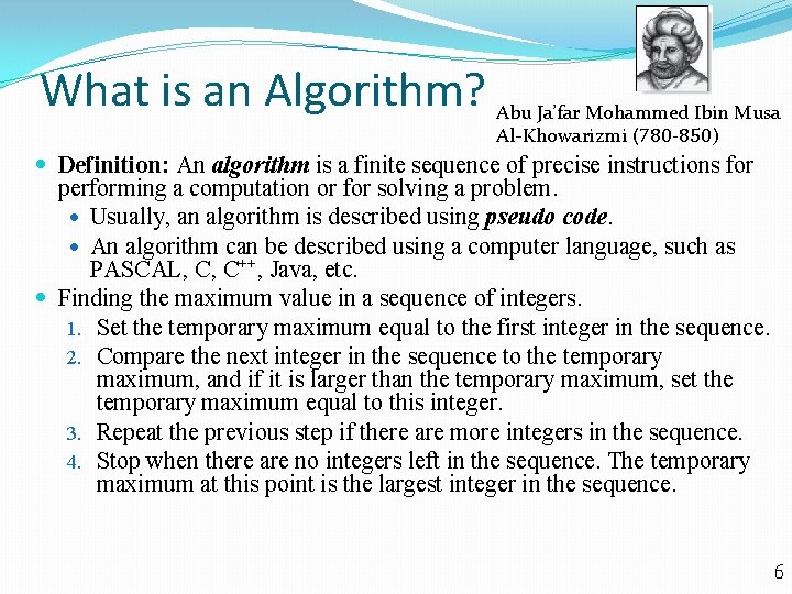
What is an Algorithm? Abu Ja’far Mohammed Ibin Musa Al-Khowarizmi (780 -850) Definition: An algorithm is a finite sequence of precise instructions for performing a computation or for solving a problem. Usually, an algorithm is described using pseudo code. An algorithm can be described using a computer language, such as PASCAL, C, C++, Java, etc. Finding the maximum value in a sequence of integers. 1. Set the temporary maximum equal to the first integer in the sequence. 2. Compare the next integer in the sequence to the temporary maximum, and if it is larger than the temporary maximum, set the temporary maximum equal to this integer. 3. Repeat the previous step if there are more integers in the sequence. 4. Stop when there are no integers left in the sequence. The temporary maximum at this point is the largest integer in the sequence. 6

Specifying Algorithms can be specified in different ways. Their steps can be described in English or in pseudo code. Pseudo code is an intermediate step between an English language description of the steps and a coding of these steps using a programming language. The form of pseudo code we use is specified in Appendix 3. It uses some of the structures found in popular languages such as C++ and Java. Programmers can use the description of an algorithm in pseudo code to construct a program in a particular language. Pseudo code helps us analyze the time required to solve a problem using an algorithm, independent of the actual programming language used to implement algorithm. 7

Properties of Algorithms Input: An algorithm has input values from a specified set. Output: From each set of input values, an algorithm produces output values from a specified set. The output values are the solution to the problem. Definiteness: The steps of an algorithm must be defined precisely. Correctness: An algorithm should produce the correct output values for each set of input values. Finiteness: An algorithm should produce the desired output after a finite number of steps for any input in the set. Effectiveness: It must be possible to perform each step of an algorithm exactly and in a finite amount of time. Generality: The procedure should be applicable for all problems of the desired form, not just for a particular set of input values. 8

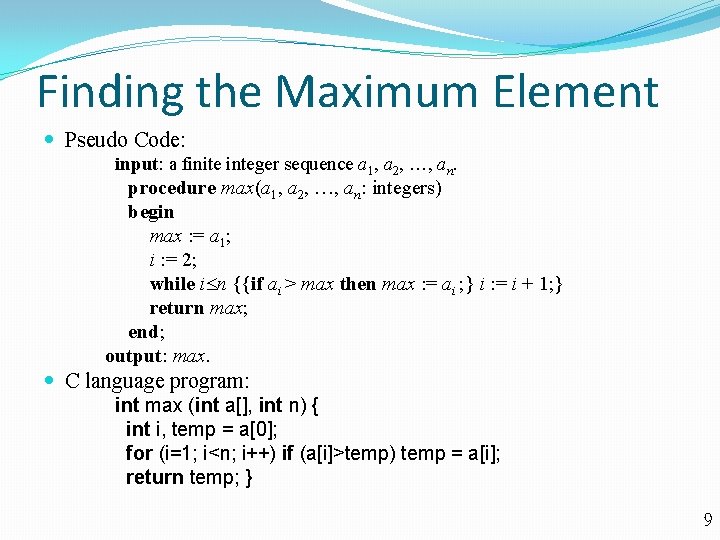
Finding the Maximum Element Pseudo Code: input: a finite integer sequence a 1, a 2, , an. procedure max(a 1, a 2, , an: integers) begin max : = a 1; i : = 2; while i n {{if ai > max then max : = ai ; } i : = i + 1; } return max; end; output: max. C language program: int max (int a[], int n) { int i, temp = a[0]; for (i=1; i<n; i++) if (a[i]>temp) temp = a[i]; return temp; } 9

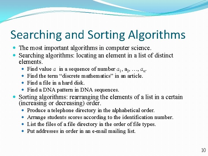
Searching and Sorting Algorithms The most important algorithms in computer science. Searching algorithms: locating an element in a list of distinct elements. Find value a in a sequence of number a 1, a 2, , an. Find the term “discrete mathematics” in an article. Find a file in a hard disk. Find a DNA pattern in DNA sequences. Sorting algorithms: rearranging the elements of a list in a certain (increasing or decreasing) order. Produce a telephone directory in the alphabetical order. Arrange students scores according to the identification number. List the files of a file directory in the order of file types. Put addresses in order in an e-mailing list. 10

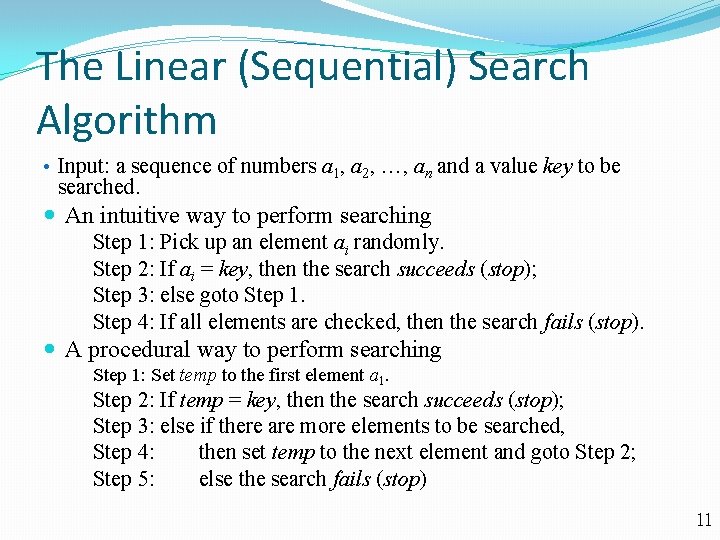
The Linear (Sequential) Search Algorithm • Input: a sequence of numbers a 1, a 2, , an and a value key to be searched. An intuitive way to perform searching Step 1: Pick up an element ai randomly. Step 2: If ai = key, then the search succeeds (stop); Step 3: else goto Step 1. Step 4: If all elements are checked, then the search fails (stop). A procedural way to perform searching Step 1: Set temp to the first element a 1. Step 2: If temp = key, then the search succeeds (stop); Step 3: else if there are more elements to be searched, Step 4: then set temp to the next element and goto Step 2; Step 5: else the search fails (stop) 11

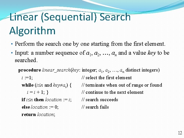
Linear (Sequential) Search Algorithm • Perform the search one by one starting from the first element. • Input: a number sequence of a 1, a 2, , an and a value key to be searched. procedure linear_search(key: integer; a 1, a 2, , an distinct integers) i : =1; while (i n and key ai) { i = i + 1; } if i n then location : = i; else location : = 0; return location; // select the first element // terminate when out of range or found // continue to the next element // search succeeds // search fails 12

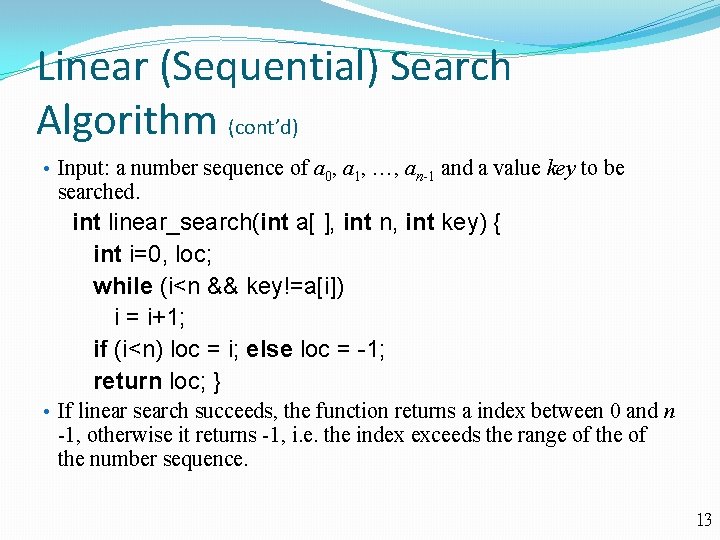
Linear (Sequential) Search Algorithm (cont’d) • Input: a number sequence of a 0, a 1, , an-1 and a value key to be searched. int linear_search(int a[ ], int n, int key) { int i=0, loc; while (i<n && key!=a[i]) i = i+1; if (i<n) loc = i; else loc = -1; return loc; } • If linear search succeeds, the function returns a index between 0 and n -1, otherwise it returns -1, i. e. the index exceeds the range of the number sequence. 13

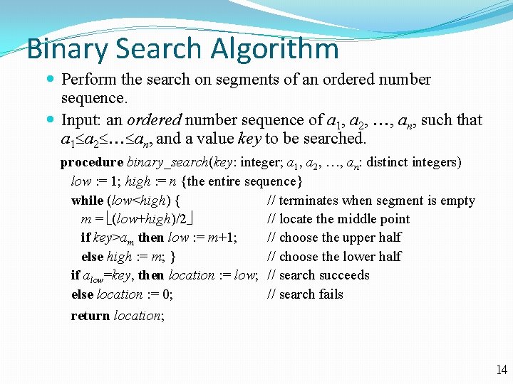
Binary Search Algorithm Perform the search on segments of an ordered number sequence. Input: an ordered number sequence of a 1, a 2, , an, such that a 1 a 2 an, and a value key to be searched. procedure binary_search(key: integer; a 1, a 2, , an: distinct integers) low : = 1; high : = n {the entire sequence} while (low<high) { // terminates when segment is empty m = (low+high)/2 // locate the middle point if key>am then low : = m+1; // choose the upper half else high : = m; } // choose the lower half if alow=key, then location : = low; // search succeeds else location : = 0; // search fails return location; 14

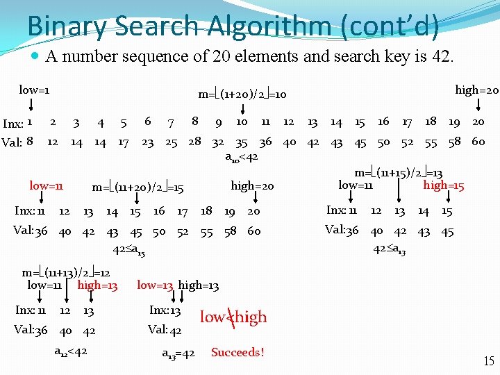
Binary Search Algorithm (cont’d) A number sequence of 20 elements and search key is 42. low=1 Inx: 1 Val: 8 2 3 4 5 12 14 14 17 12 6 7 8 9 10 11 13 14 15 16 17 18 19 20 Val: 36 40 42 43 45 50 52 55 58 60 42 a 15 m= (11+13)/2 =12 low=11 high=13 Inx: 11 13 14 15 16 17 18 19 20 Inx: 13 Val: 36 40 42 Val: 42 a 12<42 Inx: 11 12 13 14 15 Val: 36 40 42 43 45 42 a 13 low=13 high=13 13 12 12 23 25 28 32 35 36 40 42 43 45 50 52 55 58 60 a 10<42 m= (11+15)/2 =13 low=11 high=15 high=20 m= (11+20)/2 =15 low=11 Inx: 11 high=20 m= (1+20)/2 =10 a 13=42 low<high Succeeds! 15

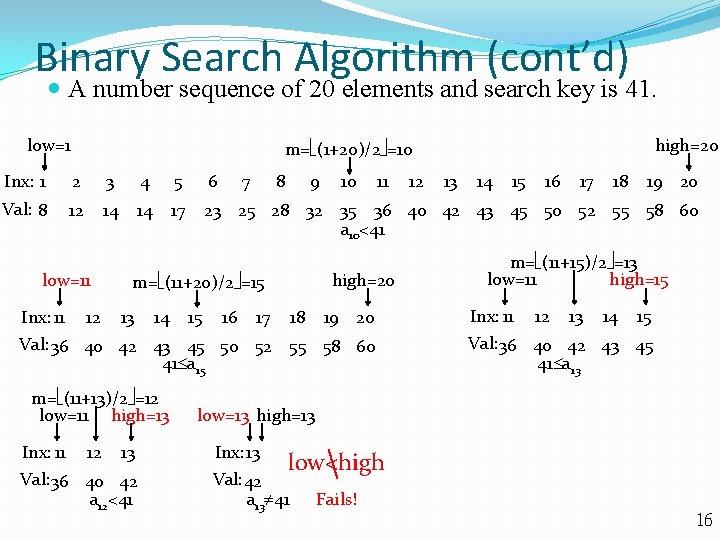
Binary Search Algorithm (cont’d) A number sequence of 20 elements and search key is 41. low=1 high=20 m= (1+20)/2 =10 Inx: 1 2 3 4 5 6 Val: 8 12 14 14 17 23 25 28 32 35 36 40 42 43 45 50 52 55 58 60 a 10<41 low=11 Inx: 11 12 7 8 9 14 15 16 11 high=20 m= (11+20)/2 =15 13 10 17 18 19 20 Val: 36 40 42 43 45 50 52 55 58 60 41 a 15 m= (11+13)/2 =12 low=11 high=13 Inx: 11 12 13 Val: 36 40 42 a 12<41 12 13 14 15 16 17 18 19 20 m= (11+15)/2 =13 low=11 high=15 Inx: 11 12 13 14 15 Val: 36 40 42 43 45 41 a 13 low=13 high=13 Inx: 13 low<high Val: 42 a 13 41 Fails! 16

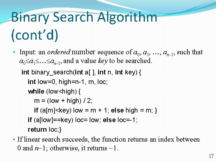
Binary Search Algorithm (cont’d) • Input: an ordered number sequence of a 0, a 1, , an-1, such that a 0 a 1 an-1, and a value key to be searched. int binary_search(int a[ ], int n, int key) { int low=0, high=n-1, m, loc; while (low<high) { m = (low + high) / 2; if (a[m]<key) low = m + 1; else high = m; } if (a[low]==key) loc= low; else loc=-1; return loc; } • If linear search succeeds, the function returns an index between 0 and n 1; otherwise, it returns 1. 17

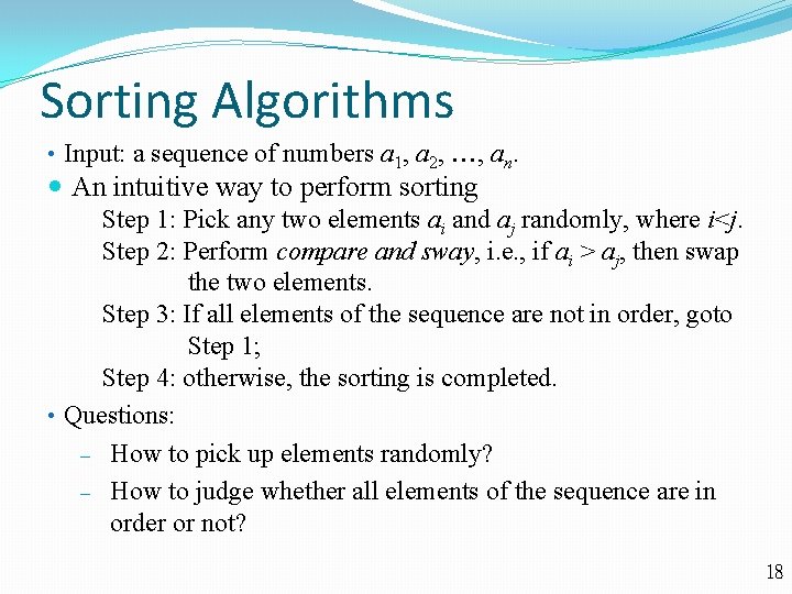
Sorting Algorithms • Input: a sequence of numbers a 1, a 2, , an. An intuitive way to perform sorting Step 1: Pick any two elements ai and aj randomly, where i<j. Step 2: Perform compare and sway, i. e. , if ai > aj, then swap the two elements. Step 3: If all elements of the sequence are not in order, goto Step 1; Step 4: otherwise, the sorting is completed. • Questions: ‒ How to pick up elements randomly? ‒ How to judge whether all elements of the sequence are in order or not? 18

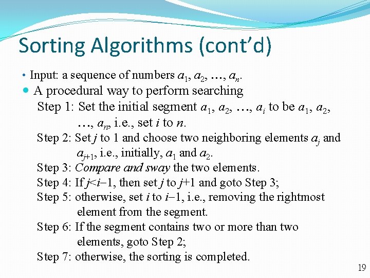
Sorting Algorithms (cont’d) • Input: a sequence of numbers a 1, a 2, , an. A procedural way to perform searching Step 1: Set the initial segment a 1, a 2, , ai to be a 1, a 2, , an, i. e. , set i to n. Step 2: Set j to 1 and choose two neighboring elements aj and aj+1, i. e. , initially, a 1 and a 2. Step 3: Compare and sway the two elements. Step 4: If j<i 1, then set j to j+1 and goto Step 3; Step 5: otherwise, set i to i 1, i. e. , removing the rightmost element from the segment. Step 6: If the segment contains two or more than two elements, goto Step 2; Step 7: otherwise, the sorting is completed. 19

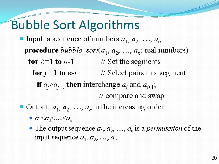
Bubble Sort Algorithms Input: a sequence of numbers a 1, a 2, , an. procedure bubble_sort(a 1, a 2, , an: real numbers) for i: =1 to n-1 // Set the segments for j: =1 to n-i // Select pairs in a segment if aj>aj+1 then interchange aj and aj+1; // compare and swap Output: a 1, a 2, , an in the increasing order. a 1 a 2 an. The output sequence a 1, a 2, , an is a permutation of the input sequence a 1, a 2, , an. 20

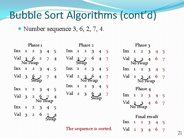
Bubble Sort Algorithms (cont’d) Number sequence 3, 6, 2, 7, 4. Inx Phase 1 1 2 3 4 5 Inx Phase 2 1 2 3 4 5 Inx 6 4 7 3 4 5 Val 2 3 4 No swap Inx 1 2 3 3 6 4 No swap 1 2 3 4 Val 2 Val 3 6 2 No swap Inx 1 2 3 7 4 4 5 Val 3 2 Swap Inx 1 2 Val 3 6 2 Swap 7 4 Val 2 7 Inx 1 2 4 5 Inx 5 Val 3 2 Inx 1 Val 3 3 6 7 4 No swap 2 3 4 5 2 6 Phase 3 1 2 3 Val 2 3 6 4 Swap 7 7 4 Swap Inx 5 6 7 4 5 3 4 6 No swap 7 Phase 4 1 2 3 4 Val 2 3 4 No swap Inx The sequence is sorted. 4 5 6 7 Final result 1 2 3 4 5 Val 2 3 4 6 7 21

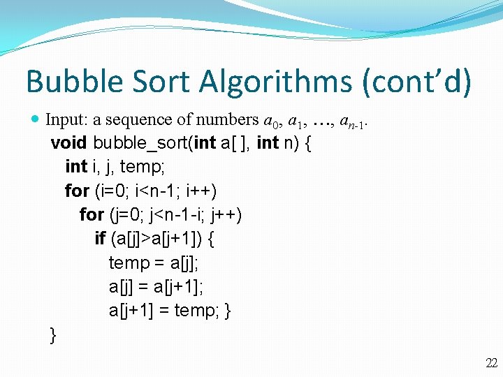
Bubble Sort Algorithms (cont’d) Input: a sequence of numbers a 0, a 1, , an-1. void bubble_sort(int a[ ], int n) { int i, j, temp; for (i=0; i<n-1; i++) for (j=0; j<n-1 -i; j++) if (a[j]>a[j+1]) { temp = a[j]; a[j] = a[j+1]; a[j+1] = temp; } } 22

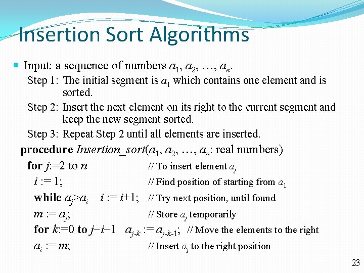
Insertion Sort Algorithms Input: a sequence of numbers a 1, a 2, , an. Step 1: The initial segment is a 1 which contains one element and is sorted. Step 2: Insert the next element on its right to the current segment and keep the new segment sorted. Step 3: Repeat Step 2 until all elements are inserted. procedure Insertion_sort(a 1, a 2, , an: real numbers) for j: =2 to n // To insert element aj i : = 1; // Find position of starting from a 1 while aj>ai i : = i+1; // Try next position, until found m : = aj; // Store aj temporarily for k: =0 to j i 1 aj-k : = aj-k-1; // Move the elements to the right ai : = m; // Insert aj to the right position 23

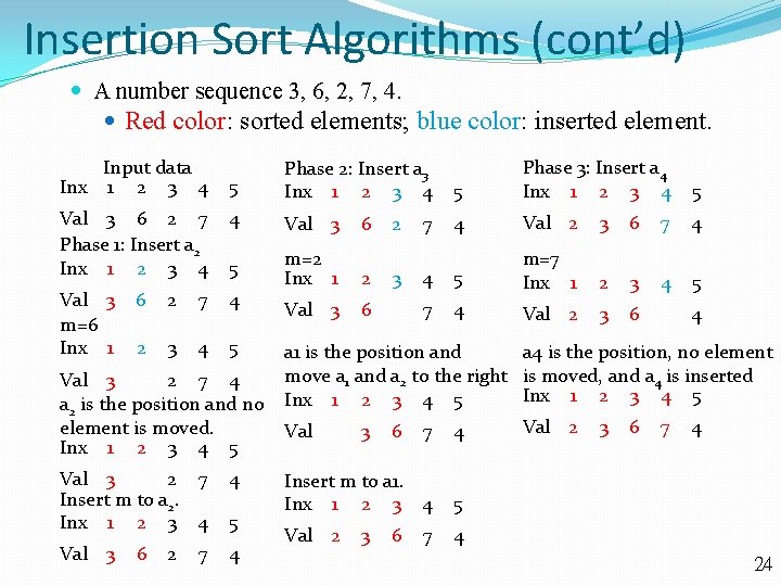
Insertion Sort Algorithms (cont’d) A number sequence 3, 6, 2, 7, 4. Red color: sorted elements; blue color: inserted element. Input data Inx 1 2 3 4 5 Phase 3: Insert a 4 Inx 1 2 3 4 5 4 Val 2 3 6 7 4 4 5 m=7 Inx 1 2 3 4 5 7 4 Val 2 3 6 5 Phase 2: Insert a 3 Inx 1 2 3 4 Val 3 6 2 7 Phase 1: Insert a 2 Inx 1 2 3 4 4 Val 3 5 Val 3 m=6 Inx 1 m=2 Inx 1 2 Val 3 6 6 2 7 4 2 3 4 5 Val 3 2 7 4 a 2 is the position and no element is moved. Inx 1 2 3 4 5 Val 3 2 7 Insert m to a 2. Inx 1 2 3 4 4 Val 3 4 6 2 7 5 6 2 3 7 4 a 4 is the position, no element a 1 is the position and move a 1 and a 2 to the right is moved, and a 4 is inserted Inx 1 2 3 4 5 Val 2 3 6 7 4 Val 3 6 7 4 Insert m to a 1. Inx 1 2 3 4 5 Val 2 4 3 6 7 24

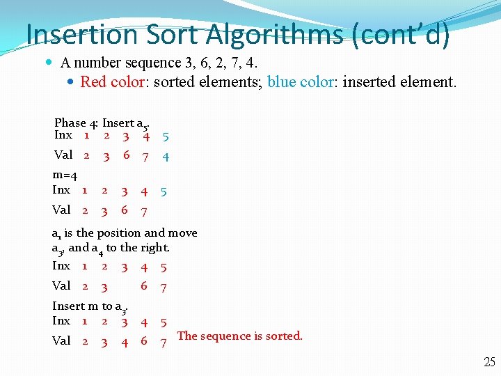
Insertion Sort Algorithms (cont’d) A number sequence 3, 6, 2, 7, 4. Red color: sorted elements; blue color: inserted element. Phase 4: Insert a 5. Inx 1 2 3 4 5 Val 2 3 6 7 4 m=4 Inx 1 2 3 4 5 Val 2 3 6 7 a 1 is the position and move a 3, and a 4 to the right. Inx 1 2 3 4 5 Val 2 3 6 7 Insert m to a 3. Inx 1 2 3 4 5 Val 2 7 The sequence is sorted. 3 4 6 25

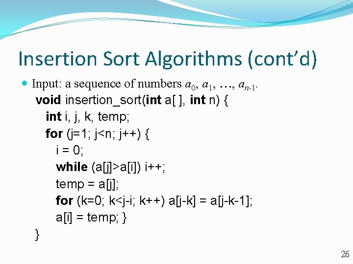
Insertion Sort Algorithms (cont’d) Input: a sequence of numbers a 0, a 1, , an-1. void insertion_sort(int a[ ], int n) { int i, j, k, temp; for (j=1; j<n; j++) { i = 0; while (a[j]>a[i]) i++; temp = a[j]; for (k=0; k<j-i; k++) a[j-k] = a[j-k-1]; a[i] = temp; } } 26

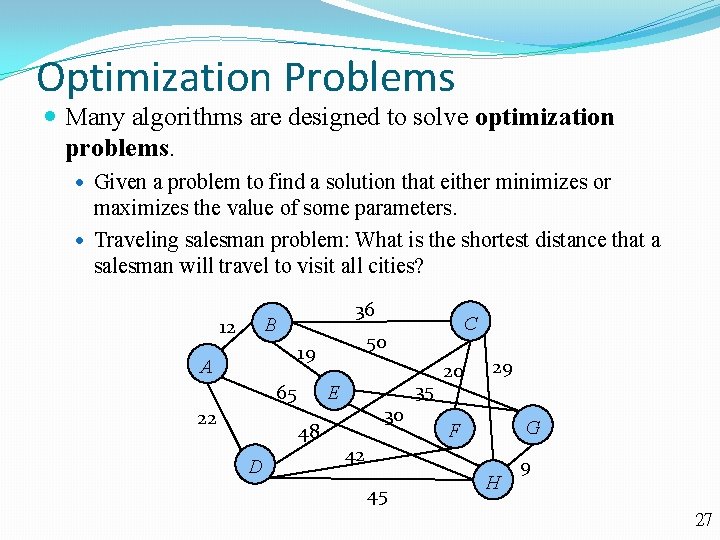
Optimization Problems Many algorithms are designed to solve optimization problems. Given a problem to find a solution that either minimizes or maximizes the value of some parameters. Traveling salesman problem: What is the shortest distance that a salesman will travel to visit all cities? 36 B 12 50 19 A 65 22 D 35 E 48 C 30 20 29 G F 42 45 H 9 27

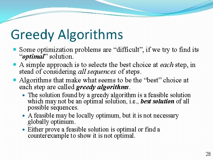
Greedy Algorithms Some optimization problems are “difficult”, if we try to find its “optimal” solution. A simple approach is to selects the best choice at each step, in stead of considering all sequences of steps. Algorithms that make what seems to be the “best” choice at each step are called greedy algorithms. The solution found by a greedy algorithm is a feasible solution which may not be an optimal solution, i. e. , best solution of all possible sequences. A feasible may be locally optimum, but it is not necessary globally optimum. Either prove a feasible solution is optimal or find a counterexample to show it is not optimal. 28

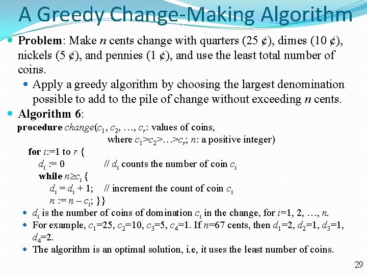
A Greedy Change-Making Algorithm Problem: Make n cents change with quarters (25 ȼ), dimes (10 ȼ), nickels (5 ȼ), and pennies (1 ȼ), and use the least total number of coins. Apply a greedy algorithm by choosing the largest denomination possible to add to the pile of change without exceeding n cents. Algorithm 6: procedure change(c 1, c 2, , cr: values of coins, where c 1>c 2> >cr; n: a positive integer) for i: =1 to r { di : = 0 // di counts the number of coin ci while n ci { di = di + 1; // increment the count of coin ci n : = n – ci; }} di is the number of coins of domination ci in the change, for i=1, 2, , n. For example, c 1=25, c 2=10, c 3=5, c 4=1. If n=67 cents, then d 1=2, d 2=1, d 3=1, d 4=2. The algorithm is an optimal solution, i. e, it uses the least number of coins. 29

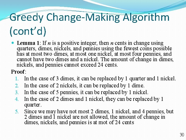
Greedy Change-Making Algorithm (cont’d) Lemma 1: If n is a positive integer, then n cents in change using quarters, dimes, nickels, and pennies using the fewest coins possible has at most two dimes, at most one nickel, at most four pennies, and cannot have two dimes and a nickel. The amount of change in dimes, nickels, and pennies cannot exceed 24 cents. Proof: 1. In the case of 3 dimes, it can be replaced by 1 quarter and 1 nickel. 2. In the case of 2 nickels, it can be replaced by 1 dime. 3. In the case of 5 pennies, it can be replaced by 1 nickel. 4. In the case of 2 dimes and 1 nickel, they can be replaced by 1 quarter. 5. Since we may have not most 2 dimes, 1 nickel, and 4 pennies, but 2 dimes and 1 nickel are not allowed, the amount of change in dimes, nickels, and pennies is at mot of 24 cents 30

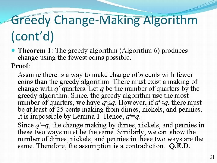
Greedy Change-Making Algorithm (cont’d) Theorem 1: The greedy algorithm (Algorithm 6) produces change using the fewest coins possible. Proof: Assume there is a way to make change of n cents with fewer coins than the greedy algorithm. There must exist a making of change with q′ quarters. Let q be the number of quarters by the greedy algorithm. Since, the greedy algorithm use the most number of quarters, we have q′ q. However, if q′<q, there must be at least of 25 cents making from dimes, nickels, and pennies. It is impossible by Lemma 1. Hence, q′=q. Since q′=q, the change making by dimes, nickels, and pennies in these two ways must be the same. Similarly, we can show the number of dimes, nickels, and pennies in these two ways are the same. Therefore, the assumption is a contradiction. Q. E. D. 31

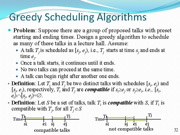
Greedy Scheduling Algorithms Problem: Suppose there a group of proposed talks with preset starting and ending times. Design a greedy algorithm to schedule as many of these talks in a lecture hall. Assume: A talk Tj is scheduled as [sj, ej), i. e. , Tj starts at time sj and ends at time ej. Once a talk starts, it continues until it ends. No two talks can proceed at the same time. A talk can begin right after another one ends. • Definition: Let Ti and Tj be two distinct talks with schedules [si, ei) and [sj, ej), respectively, Ti and Tj are compatible if si ej or sj ei, i. e. , [si, ei) [sj, ej)=. • Definition: Let S be a set of talks, talk Ti is compatible with S, if Ti is compatible with Tj, for all Tj S Ti Time si Tj ei sj ej compatible talks Ti Time Tj si sj ei ej not compatible talks 32

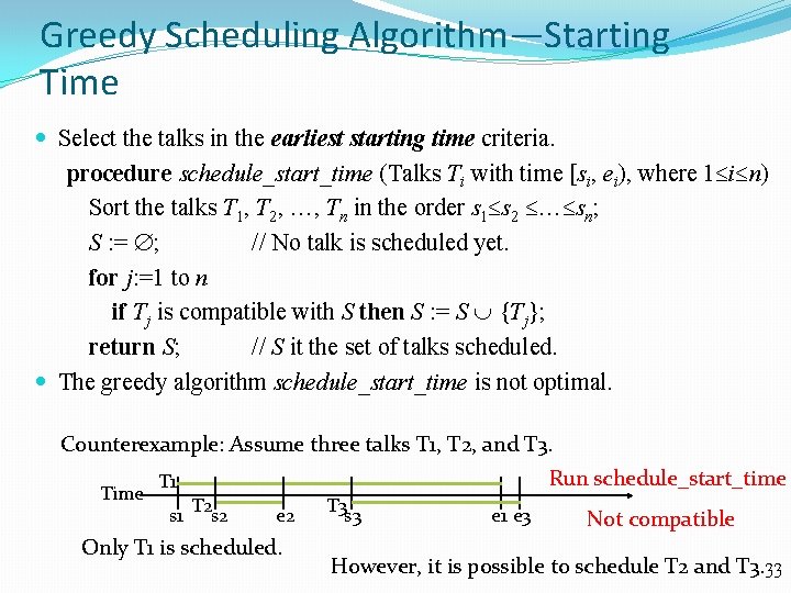
Greedy Scheduling Algorithm—Starting Time Select the talks in the earliest starting time criteria. procedure schedule_start_time (Talks Ti with time [si, ei), where 1 i n) Sort the talks T 1, T 2, , Tn in the order s 1 s 2 sn; S : = ; // No talk is scheduled yet. for j: =1 to n if Tj is compatible with S then S : = S {Tj}; return S; // S it the set of talks scheduled. The greedy algorithm schedule_start_time is not optimal. Counterexample: Assume three talks T 1, T 2, and T 3. Time Run schedule_start_time T 1 s 1 T 2 s 2 e 2 Only T 1 is scheduled. T 3 s 3 e 1 e 3 Not compatible However, it is possible to schedule T 2 and T 3. 33

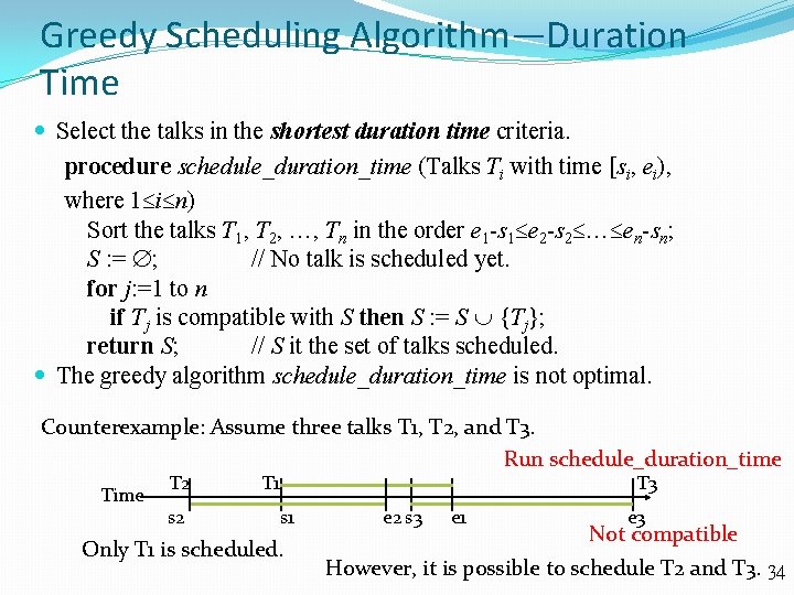
Greedy Scheduling Algorithm—Duration Time Select the talks in the shortest duration time criteria. procedure schedule_duration_time (Talks Ti with time [si, ei), where 1 i n) Sort the talks T 1, T 2, , Tn in the order e 1 -s 1 e 2 -s 2 en-sn; S : = ; // No talk is scheduled yet. for j: =1 to n if Tj is compatible with S then S : = S {Tj}; return S; // S it the set of talks scheduled. The greedy algorithm schedule_duration_time is not optimal. Counterexample: Assume three talks T 1, T 2, and T 3. Run schedule_duration_time T 2 s 2 T 1 T 3 s 1 Only T 1 is scheduled. e 2 s 3 e 1 e 3 Not compatible However, it is possible to schedule T 2 and T 3. 34

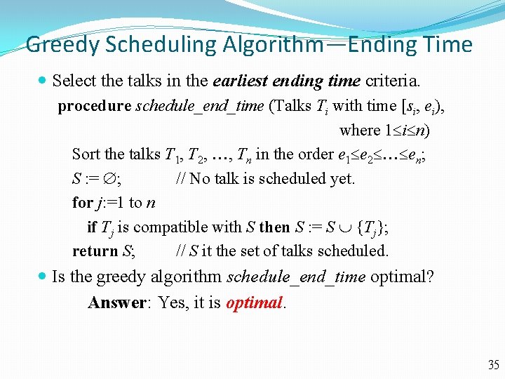
Greedy Scheduling Algorithm—Ending Time Select the talks in the earliest ending time criteria. procedure schedule_end_time (Talks Ti with time [si, ei), where 1 i n) Sort the talks T 1, T 2, , Tn in the order e 1 e 2 en; S : = ; // No talk is scheduled yet. for j: =1 to n if Tj is compatible with S then S : = S {Tj}; return S; // S it the set of talks scheduled. Is the greedy algorithm schedule_end_time optimal? Answer: Yes, it is optimal. 35

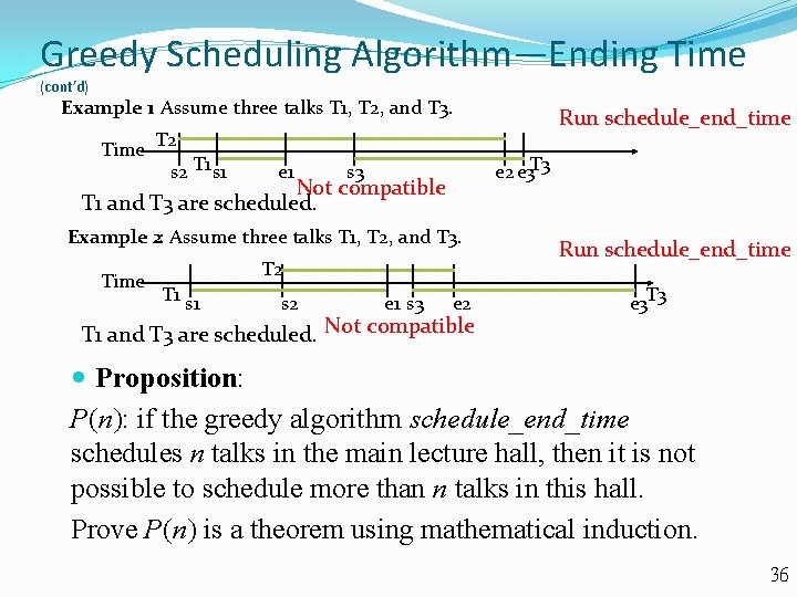
Greedy Scheduling Algorithm—Ending Time (cont’d) Example 1: Assume three talks T 1, T 2, and T 3. Time T 2 s 2 T 1 s 1 e 2 e 3 T 3 s 3 Not compatible T 1 and T 3 are scheduled. Example 2: Assume three talks T 1, T 2, and T 3. Time T 2 T 1 s 2 e 1 s 3 Run schedule_end_time e 2 T 1 and T 3 are scheduled. Not compatible Run schedule_end_time e 3 T 3 Proposition: P(n): if the greedy algorithm schedule_end_time schedules n talks in the main lecture hall, then it is not possible to schedule more than n talks in this hall. Prove P(n) is a theorem using mathematical induction. 36

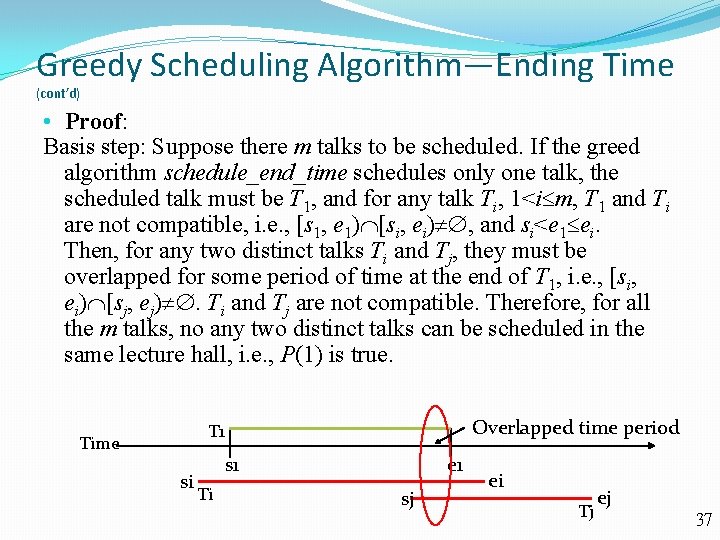
Greedy Scheduling Algorithm—Ending Time (cont’d) • Proof: Basis step: Suppose there m talks to be scheduled. If the greed algorithm schedule_end_time schedules only one talk, the scheduled talk must be T 1, and for any talk Ti, 1<i m, T 1 and Ti are not compatible, i. e. , [s 1, e 1) [si, ei) , and si<e 1 ei. Then, for any two distinct talks Ti and Tj, they must be overlapped for some period of time at the end of T 1, i. e. , [si, ei) [sj, ej) . Ti and Tj are not compatible. Therefore, for all the m talks, no any two distinct talks can be scheduled in the same lecture hall, i. e. , P(1) is true. Overlapped time period T 1 Time si s 1 Ti e 1 sj ei Tj ej 37

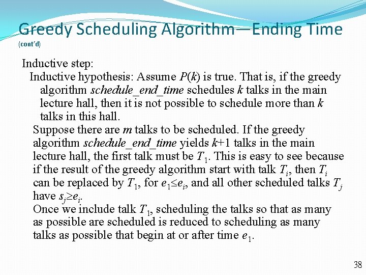
Greedy Scheduling Algorithm—Ending Time (cont’d) Inductive step: Inductive hypothesis: Assume P(k) is true. That is, if the greedy algorithm schedule_end_time schedules k talks in the main lecture hall, then it is not possible to schedule more than k talks in this hall. Suppose there are m talks to be scheduled. If the greedy algorithm schedule_end_time yields k+1 talks in the main lecture hall, the first talk must be T 1. This is easy to see because if the result of the greedy algorithm start with talk Ti, then Ti can be replaced by T 1, for e 1 ei, and all other scheduled talks Tj have sj ei. Once we include talk T 1, scheduling the talks so that as many as possible are scheduled is reduced to scheduling as many talks as possible that begin at or after time e 1. 38

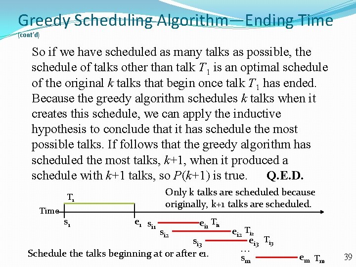
Greedy Scheduling Algorithm—Ending Time (cont’d) So if we have scheduled as many talks as possible, the schedule of talks other than talk T 1 is an optimal schedule of the original k talks that begin once talk T 1 has ended. Because the greedy algorithm schedules k talks when it creates this schedule, we can apply the inductive hypothesis to conclude that it has schedule the most possible talks. If follows that the greedy algorithm has scheduled the most talks, k+1, when it produced a schedule with k+1 talks, so P(k+1) is true. Q. E. D. Only k talks are scheduled because originally, k+1 talks are scheduled. T 1 Time s 1 e 1 si 2 ei 1 Ti 1 si 3 Schedule the talks beginning at or after e 1. ei 2 Ti 2 ei 3 Ti 3 sm em T m 39

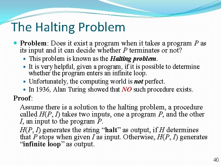
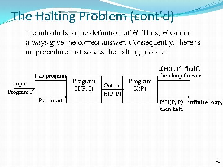
The Halting Problem: Does it exist a program when it takes a program P as its input and it can decide whether P terminates or not? This problem is known as the Halting problem. It is very helpful, given a program, if it is possible to determine whether the program enters an infinite loop. Unfortunately, the computing world is not perfect. In 1936, Alan Turing showed that NO such procedure exists. Proof: Assume there is a solution to the halting problem, a procedure called H(P, I) takes two inputs, one a program P, and the other I, an input to the program P. H(P, I) generates the string “halt” as output, if H determines that P stops when given I as input. Otherwise, H(P, I) generates “infinite loop” as output. 40

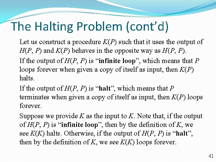
The Halting Problem (cont’d) Let us construct a procedure K(P) such that it uses the output of H(P, P) and K(P) behaves in the opposite way as H(P, P). If the output of H(P, P) is “infinite loop”, which means that P loops forever when given a copy of itself as input, then K(P) halts. If the output of H(P, P) is “halt”, which means that P terminates when given a copy of itself as input, then K(P) loops forever. Suppose we provide K as the input to K. Note that, if the output of H(P, P) is “infinite loop”, then by the definition of K, we see K(K) halts. Otherwise, if the output of H(P, P) is “halt”, then by the definition of K, we see K(K) loops forever. 41

The Halting Problem (cont’d) It contradicts to the definition of H. Thus, H cannot always give the correct answer. Consequently, there is no procedure that solves the halting problem. P as program Input Program P P as input Program H(P, I) Output H(P, P) Program K(P) If H(P, P)=“halt”, then loop forever If H(P, P)=“infinite loop”, then halt. 42

The Growth of Functions Section 3. 2 43

Section Summary Donald E. Knuth (Born 1938) Big-O Notation Big-O Estimates for Important Functions Big-Omega and Big-Theta Notation Edmund Landau (1877 -1938) Paul Gustav Heinrich Bachmann (1837 -1920) 44

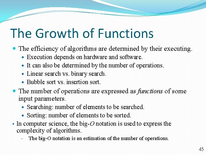
The Growth of Functions The efficiency of algorithms are determined by their executing. Execution depends on hardware and software. It can also be determined by the number of operations. Linear search vs. binary search. Bubble sort vs. insertion sort. The number of operations are expressed as functions of some input parameters. Searching: number of elements to be searched. Sorting: number of elements to be sorted. • In computer science, the big-O notation is used to express the complexity of algorithms. − The big-O notation is an estimation of the number of operations. 45

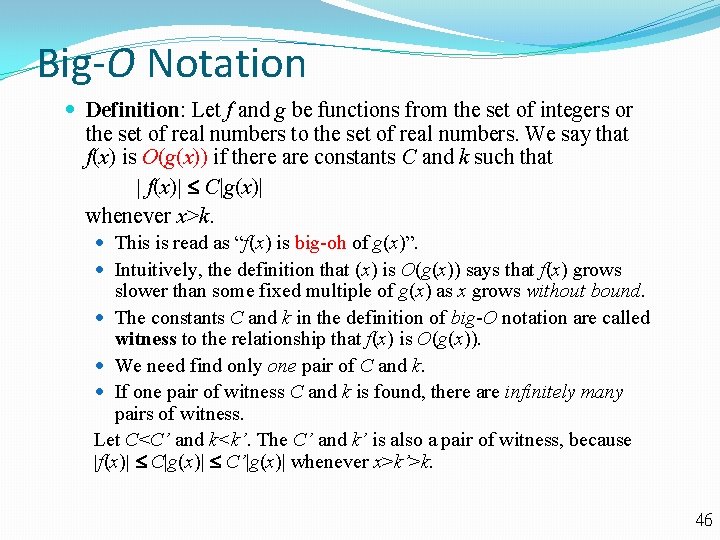
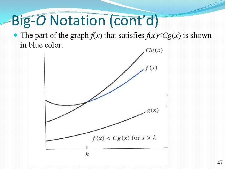
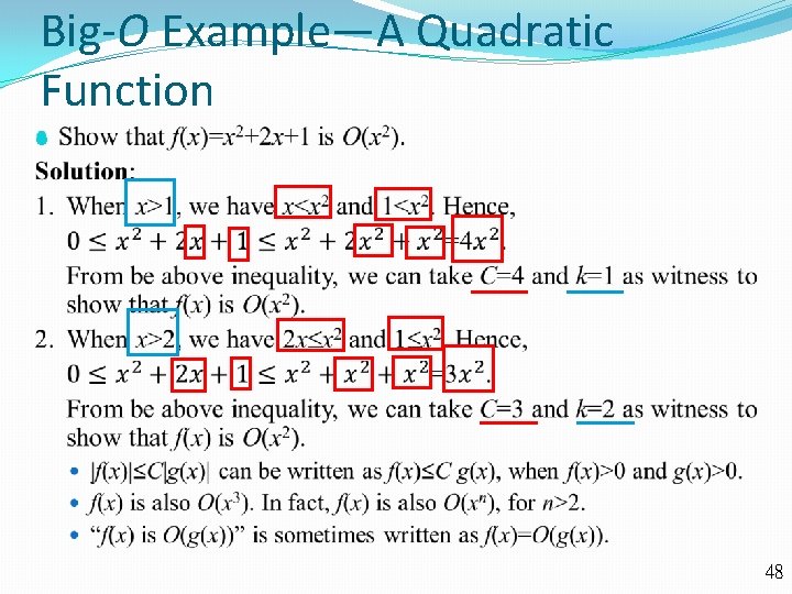
Big-O Notation Definition: Let f and g be functions from the set of integers or the set of real numbers to the set of real numbers. We say that f(x) is O(g(x)) if there are constants C and k such that | f(x)| C|g(x)| whenever x>k. This is read as “f(x) is big-oh of g(x)”. Intuitively, the definition that (x) is O(g(x)) says that f(x) grows slower than some fixed multiple of g(x) as x grows without bound. The constants C and k in the definition of big-O notation are called witness to the relationship that f(x) is O(g(x)). We need find only one pair of C and k. If one pair of witness C and k is found, there are infinitely many pairs of witness. Let C<C’ and k<k’. The C’ and k’ is also a pair of witness, because |f(x)| C|g(x)| C’|g(x)| whenever x>k’>k. 46

Big-O Notation (cont’d) The part of the graph f(x) that satisfies f(x)<Cg(x) is shown in blue color. 47

Big-O Example—A Quadratic Function 48

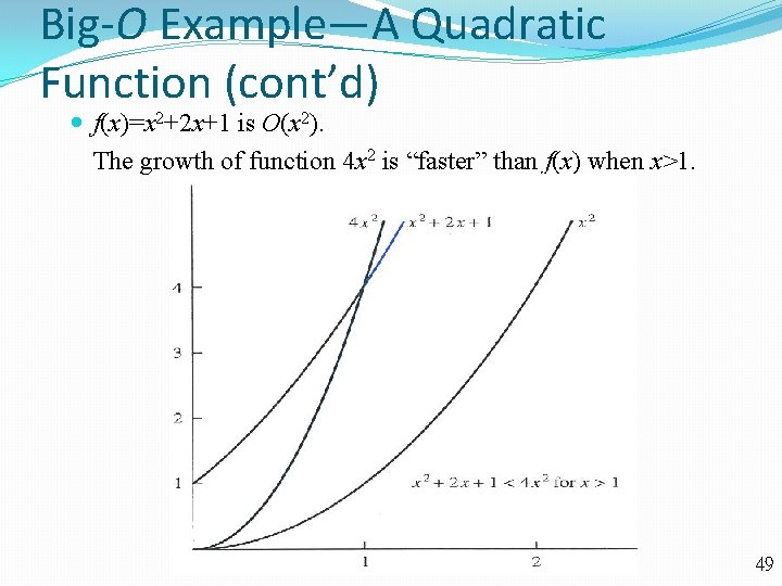
Big-O Example—A Quadratic Function (cont’d) f(x)=x 2+2 x+1 is O(x 2). The growth of function 4 x 2 is “faster” than f(x) when x>1. 49

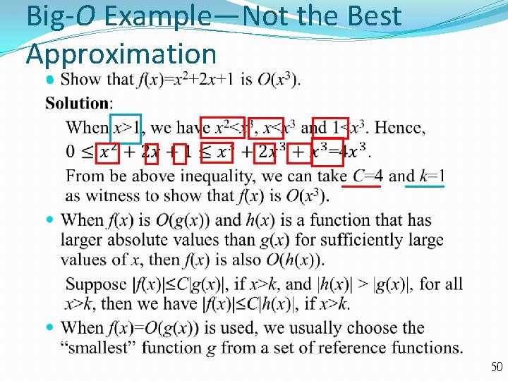
Big-O Example—Not the Best Approximation 50

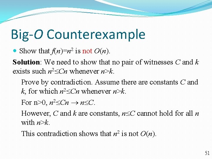
Big-O Counterexample Show that f(n)=n 2 is not O(n). Solution: We need to show that no pair of witnesses C and k exists such n 2 Cn whenever n>k. Prove by contradiction. Assume there are constants C and k, for which n 2 Cn whenever n>k. For n>0, n 2 Cn n C. However, C and k are constants, n C cannot hold for all n with n>k. This contradiction shows that n 2 is not O(n). 51

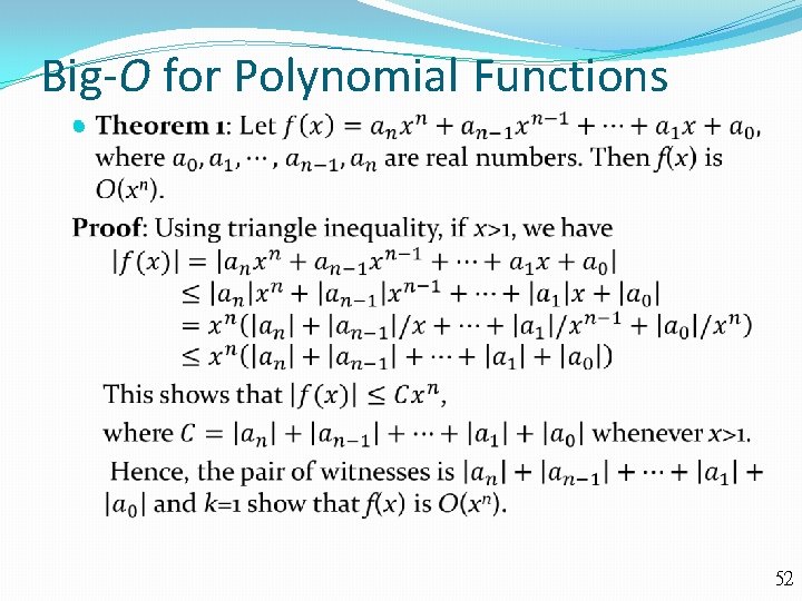
Big-O for Polynomial Functions 52

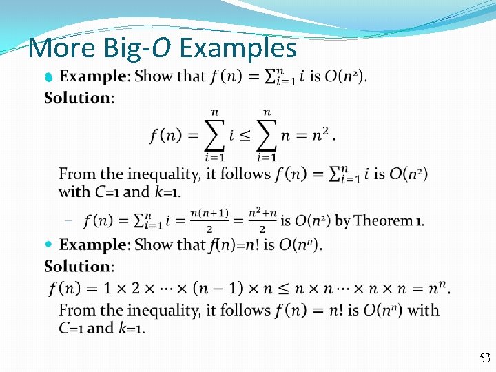
More Big-O Examples 53

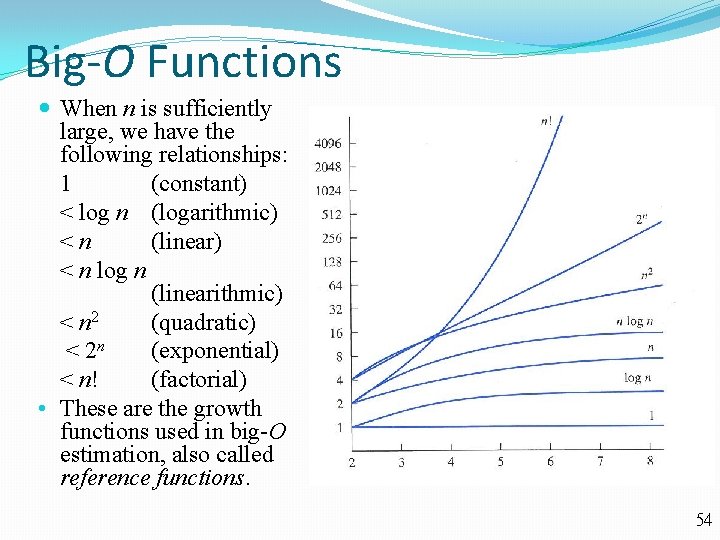
Big-O Functions When n is sufficiently large, we have the following relationships: 1 (constant) < log n (logarithmic) <n (linear) < n log n (linearithmic) < n 2 (quadratic) < 2 n (exponential) < n! (factorial) • These are the growth functions used in big-O estimation, also called reference functions. 54

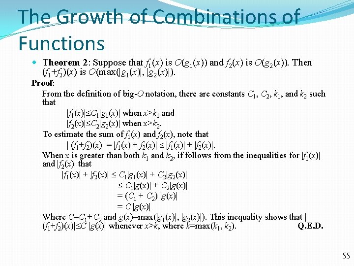
The Growth of Combinations of Functions Theorem 2: Suppose that f 1(x) is O(g 1(x)) and f 2(x) is O(g 2(x)). Then (f 1+f 2)(x) is O(max(|g 1(x)|, |g 2(x)|). Proof: From the definition of big-O notation, there are constants C 1, C 2, k 1, and k 2 such that |f 1(x)| C 1|g 1(x)| when x>k 1 and |f 2(x)| C 2|g 2(x)| when x>k 2. To estimate the sum of f 1(x) and f 2(x), note that | (f 1+f 2)(x)| = |f 1(x) + f 2(x)| |f 1(x)| + |f 2(x)|. When x is greater than both k 1 and k 2, if follows from the inequalities for |f 1(x)| and |f 2(x)| that |f 1(x)| + |f 2(x)| C 1|g 1(x)| + C 2|g 2(x)| C 1|g(x)| + C 2|g(x)| = (C 1 + C 2) |g(x)| = C |g(x)| Where C=C 1+C 2 and g(x)=max(|g 1(x)|, |g 2(x)|). This inequality shows that | (f 1+f 2)(x)| C |g(x)| whenever x>k, where k=max(k 1, k 2). Q. E. D. 55

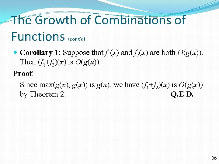
The Growth of Combinations of Functions (cont’d) Corollary 1: Suppose that f 1(x) and f 2(x) are both O(g(x)). Then (f 1+f 2)(x) is O(g(x)). Proof: Since max(g(x), g(x)) is g(x), we have (f 1+f 2)(x) is O(g(x)) by Theorem 2. Q. E. D. 56

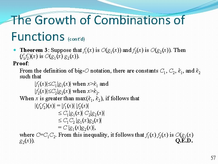
The Growth of Combinations of Functions (cont’d) Theorem 3: Suppose that f 1(x) is O(g 1(x)) and f 2(x) is O(g 2(x)). Then (f 1 f 2)(x) is O(g 1(x) g 2(x)). Proof: From the definition of big-O notation, there are constants C 1, C 2, k 1, and k 2 such that |f 1(x)| C 1|g 1(x)| when x>k 1 and |f 2(x)| C 2|g 2(x)| when x>k 2. When x is greater than max(k 1, k 2), if follows that |(f 1 f 2)(x)| = |f 1(x)| |f 2(x)| C 1|g 1(x)| C 2|g 2(x)| C 1 C 2 |g 1(x)g 2(x)| = C |g 1(x)g 2(x)|, where C=C 1 C 2. From this inequality, it follows that f 1(x) f 2(x) is O(g 1(x) g 2(x)). Q. E. D. 57

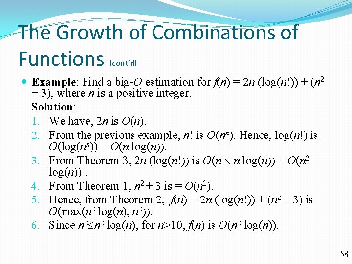
The Growth of Combinations of Functions (cont’d) Example: Find a big-O estimation for f(n) = 2 n (log(n!)) + (n 2 + 3), where n is a positive integer. Solution: 1. We have, 2 n is O(n). 2. From the previous example, n! is O(nn). Hence, log(n!) is O(log(nn)) = O(n log(n)). 3. From Theorem 3, 2 n (log(n!)) is O(n n log(n)) = O(n 2 log(n)). 4. From Theorem 1, n 2 + 3 is = O(n 2). 5. Hence, from Theorem 2, f(n) = 2 n (log(n!)) + (n 2 + 3) is O(max(n 2 log(n), n 2)). 6. Since n 2 log(n), for n>10, f(n) is O(n 2 log(n)). 58

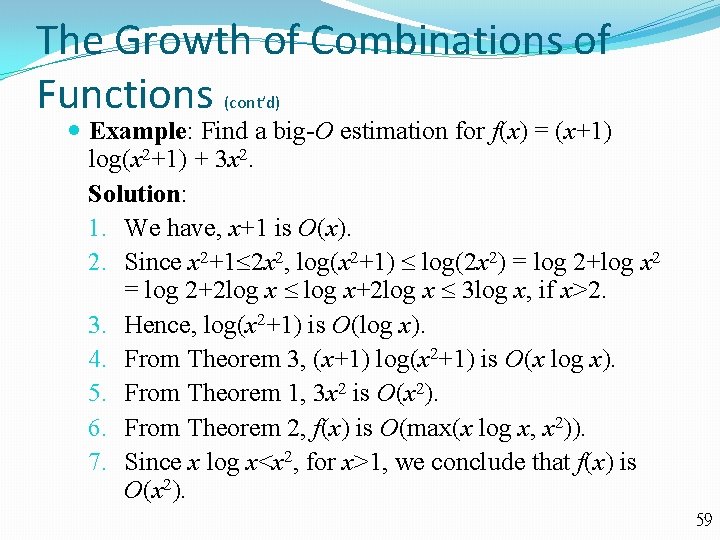
The Growth of Combinations of Functions (cont’d) Example: Find a big-O estimation for f(x) = (x+1) log(x 2+1) + 3 x 2. Solution: 1. We have, x+1 is O(x). 2. Since x 2+1 2 x 2, log(x 2+1) log(2 x 2) = log 2+log x 2 = log 2+2 log x log x+2 log x 3 log x, if x>2. 3. Hence, log(x 2+1) is O(log x). 4. From Theorem 3, (x+1) log(x 2+1) is O(x log x). 5. From Theorem 1, 3 x 2 is O(x 2). 6. From Theorem 2, f(x) is O(max(x log x, x 2)). 7. Since x log x<x 2, for x>1, we conclude that f(x) is O(x 2). 59

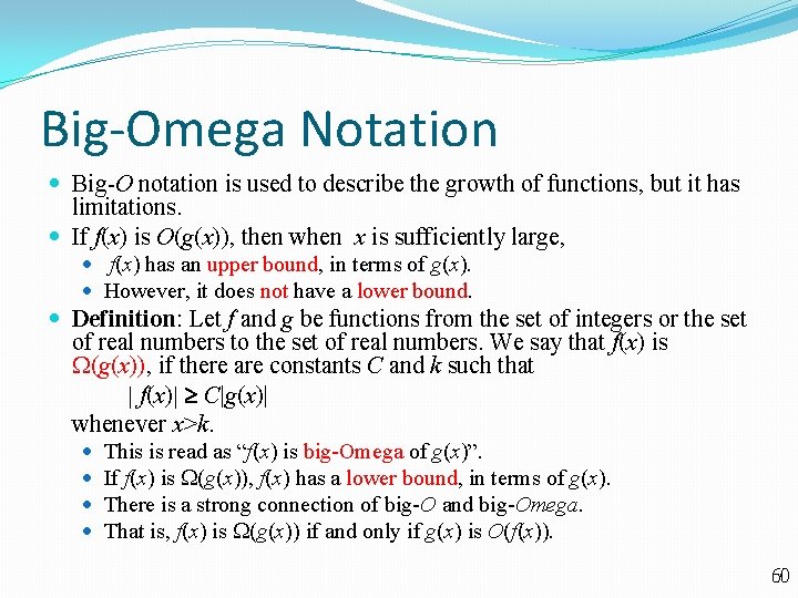
Big-Omega Notation Big-O notation is used to describe the growth of functions, but it has limitations. If f(x) is O(g(x)), then when x is sufficiently large, f(x) has an upper bound, in terms of g(x). However, it does not have a lower bound. Definition: Let f and g be functions from the set of integers or the set of real numbers to the set of real numbers. We say that f(x) is (g(x)), if there are constants C and k such that | f(x)| C|g(x)| whenever x>k. This is read as “f(x) is big-Omega of g(x)”. If f(x) is (g(x)), f(x) has a lower bound, in terms of g(x). There is a strong connection of big-O and big-Omega. That is, f(x) is (g(x)) if and only if g(x) is O(f(x)). 60

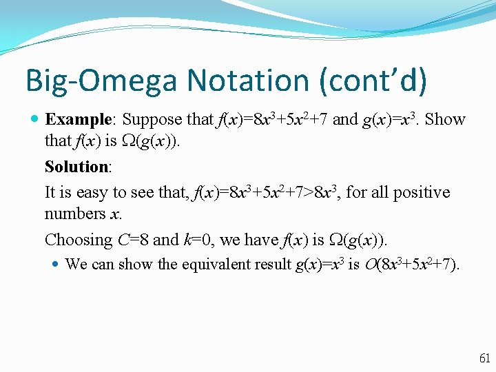
Big-Omega Notation (cont’d) Example: Suppose that f(x)=8 x 3+5 x 2+7 and g(x)=x 3. Show that f(x) is (g(x)). Solution: It is easy to see that, f(x)=8 x 3+5 x 2+7>8 x 3, for all positive numbers x. Choosing C=8 and k=0, we have f(x) is (g(x)). We can show the equivalent result g(x)=x 3 is O(8 x 3+5 x 2+7). 61

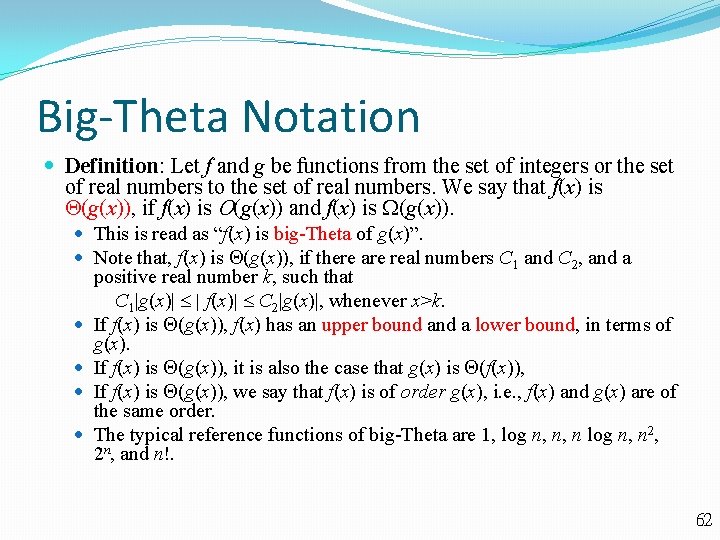
Big-Theta Notation Definition: Let f and g be functions from the set of integers or the set of real numbers to the set of real numbers. We say that f(x) is (g(x)), if f(x) is O(g(x)) and f(x) is (g(x)). This is read as “f(x) is big-Theta of g(x)”. Note that, f(x) is (g(x)), if there are real numbers C 1 and C 2, and a positive real number k, such that C 1|g(x)| | f(x)| C 2|g(x)|, whenever x>k. If f(x) is (g(x)), f(x) has an upper bound a lower bound, in terms of g(x). If f(x) is (g(x)), it is also the case that g(x) is (f(x)), If f(x) is (g(x)), we say that f(x) is of order g(x), i. e. , f(x) and g(x) are of the same order. The typical reference functions of big-Theta are 1, log n, n, n log n, n 2, 2 n, and n!. 62

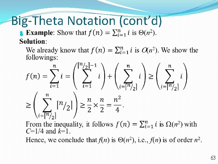
Big-Theta Notation (cont’d) 63

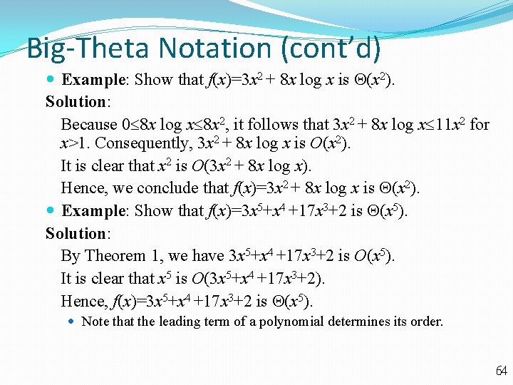
Big-Theta Notation (cont’d) Example: Show that f(x)=3 x 2 + 8 x log x is (x 2). Solution: Because 0 8 x log x 8 x 2, it follows that 3 x 2 + 8 x log x 11 x 2 for x>1. Consequently, 3 x 2 + 8 x log x is O(x 2). It is clear that x 2 is O(3 x 2 + 8 x log x). Hence, we conclude that f(x)=3 x 2 + 8 x log x is (x 2). Example: Show that f(x)=3 x 5+x 4 +17 x 3+2 is (x 5). Solution: By Theorem 1, we have 3 x 5+x 4 +17 x 3+2 is O(x 5). It is clear that x 5 is O(3 x 5+x 4 +17 x 3+2). Hence, f(x)=3 x 5+x 4 +17 x 3+2 is (x 5). Note that the leading term of a polynomial determines its order. 64

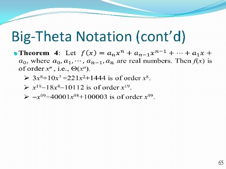
Big-Theta Notation (cont’d) 65

Complexity of Algorithms Section 3. 3 66

Section Summary Time Complexity Worst-Case Complexity Algorithmic Paradigms Understanding the Complexity of Algorithms 67

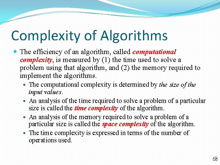
Complexity of Algorithms The efficiency of an algorithm, called computational complexity, is measured by (1) the time used to solve a problem using that algorithm, and (2) the memory required to implement the algorithms. The computational complexity is determined by the size of the input values. An analysis of the time required to solve a problem of a particular size is called the time complexity of the algorithm. An analysis of the memory required to solve a problem of a particular size is called the space complexity of the algorithm. The time complexity is expressed in terms of the number of operations used. 68

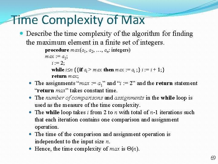
Time Complexity of Max Describe the time complexity of the algorithm for finding the maximum element in a finite set of integers. procedure max(a 1, a 2, , an: integers) max : = a 1; i : = 2; while i n {{if ai > max then max : = ai ; } i : = i + 1; } return max; The assignments “max : = a 1” and “i : = 2” and the return statement “return max” takes constant time. The number of comparisons and assignments in the while loop is used as the measure of the time complexity. The while loop takes i from 2 to n with total of n-1 iterations such that each iteration contains one comparison and assignment operation. The time of the comparison and assignment operation is independent to the input size n. Hence, the time complexity of max is (n). 69

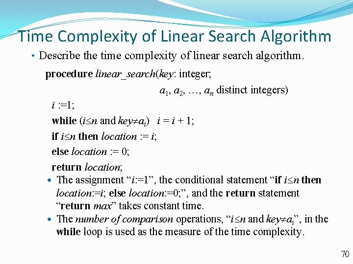
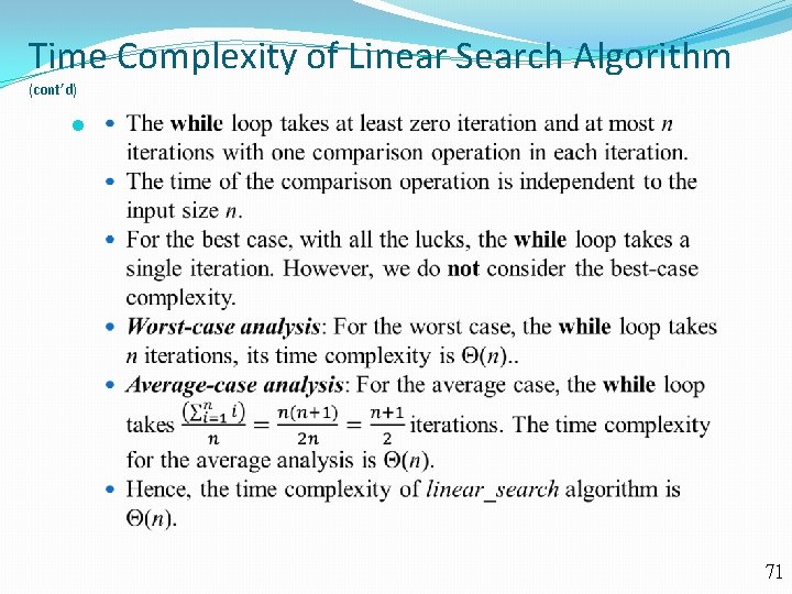
Time Complexity of Linear Search Algorithm • Describe the time complexity of linear search algorithm. procedure linear_search(key: integer; a 1, a 2, , an distinct integers) i : =1; while (i n and key ai) i = i + 1; if i n then location : = i; else location : = 0; return location; The assignment “i: =1”, the conditional statement “if i n then location: =i; else location: =0; ”, and the return statement “return max” takes constant time. The number of comparison operations, “i n and key ai”, in the while loop is used as the measure of the time complexity. 70

Time Complexity of Linear Search Algorithm (cont’d) 71

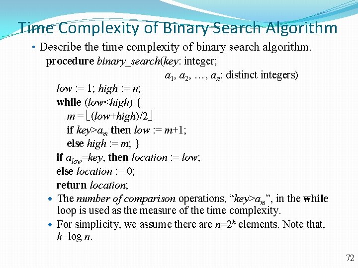
Time Complexity of Binary Search Algorithm • Describe the time complexity of binary search algorithm. procedure binary_search(key: integer; a 1, a 2, , an: distinct integers) low : = 1; high : = n; while (low<high) { m = (low+high)/2 if key>am then low : = m+1; else high : = m; } if alow=key, then location : = low; else location : = 0; return location; The number of comparison operations, “key>am”, in the while loop is used as the measure of the time complexity. For simplicity, we assume there are n=2 k elements. Note that, k=log n. 72

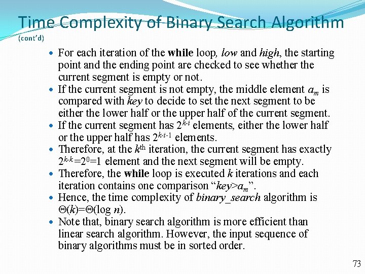
Time Complexity of Binary Search Algorithm (cont’d) For each iteration of the while loop, low and high, the starting point and the ending point are checked to see whether the current segment is empty or not. If the current segment is not empty, the middle element am is compared with key to decide to set the next segment to be either the lower half or the upper half of the current segment. If the current segment has 2 k-i elements, either the lower half or the upper half has 2 k-i-1 elements. Therefore, at the kth iteration, the current segment has exactly 2 k-k =20=1 element and the next segment will be empty. Therefore, the while loop is executed k iterations and each iteration contains one comparison “key>am”. Hence, the time complexity of binary_search algorithm is (k)= (log n). Note that, binary search algorithm is more efficient than linear search algorithm. However, the input sequence of binary algorithms must be in sorted order. 73

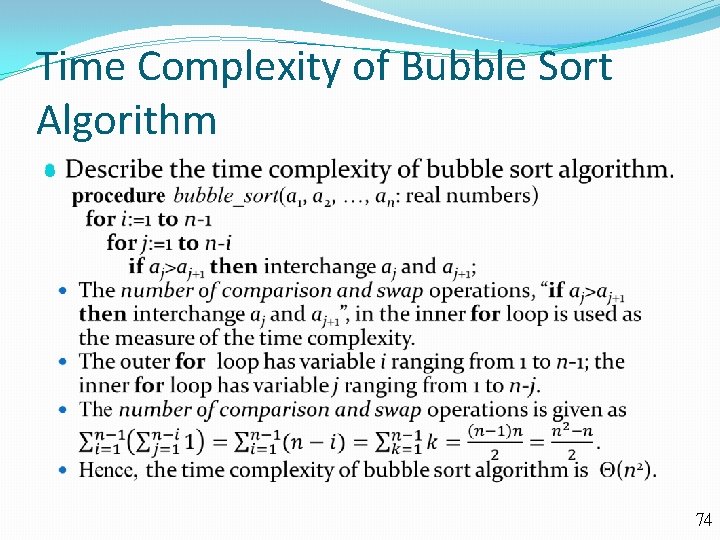
Time Complexity of Bubble Sort Algorithm 74

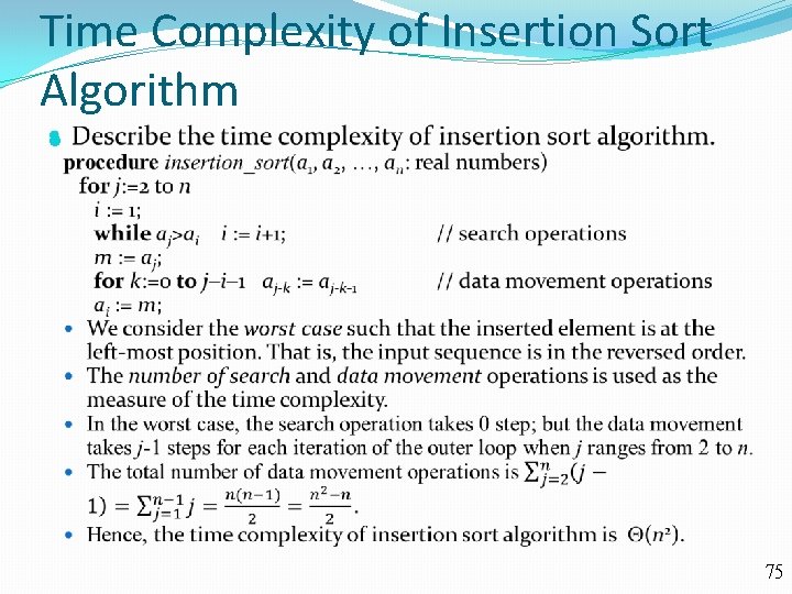
Time Complexity of Insertion Sort Algorithm 75

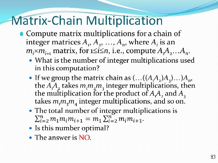
Matrix-Chain Multiplication 83

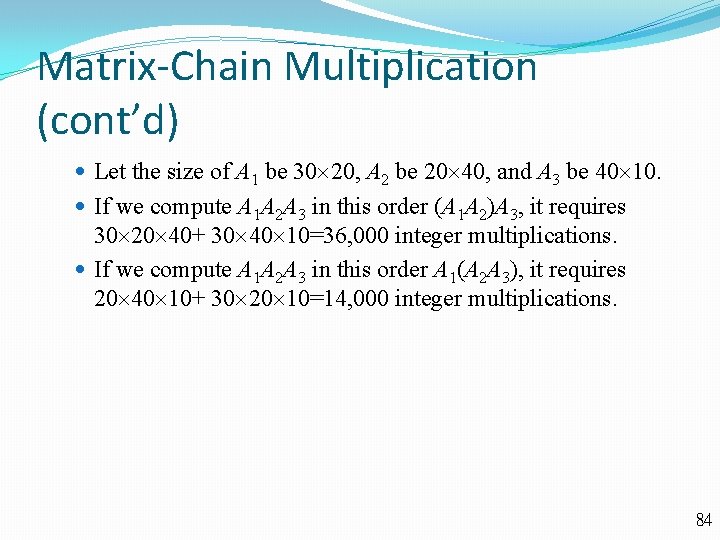
Matrix-Chain Multiplication (cont’d) Let the size of A 1 be 30 20, A 2 be 20 40, and A 3 be 40 10. If we compute A 1 A 2 A 3 in this order (A 1 A 2)A 3, it requires 30 20 40+ 30 40 10=36, 000 integer multiplications. If we compute A 1 A 2 A 3 in this order A 1(A 2 A 3), it requires 20 40 10+ 30 20 10=14, 000 integer multiplications. 84

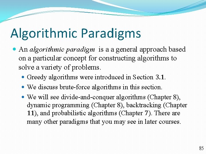
Algorithmic Paradigms An algorithmic paradigm is a a general approach based on a particular concept for constructing algorithms to solve a variety of problems. Greedy algorithms were introduced in Section 3. 1. We discuss brute-force algorithms in this section. We will see divide-and-conquer algorithms (Chapter 8), dynamic programming (Chapter 8), backtracking (Chapter 11), and probabilistic algorithms (Chapter 7). There are many other paradigms that you may see in later courses. 85

Brute-Force Algorithms A brute-force algorithm is solved in the most straightforward manner, without taking advantage of any ideas that can make the algorithm more efficient. Brute-force algorithms we have previously seen are sequential search, bubble sort, and insertion sort. 86

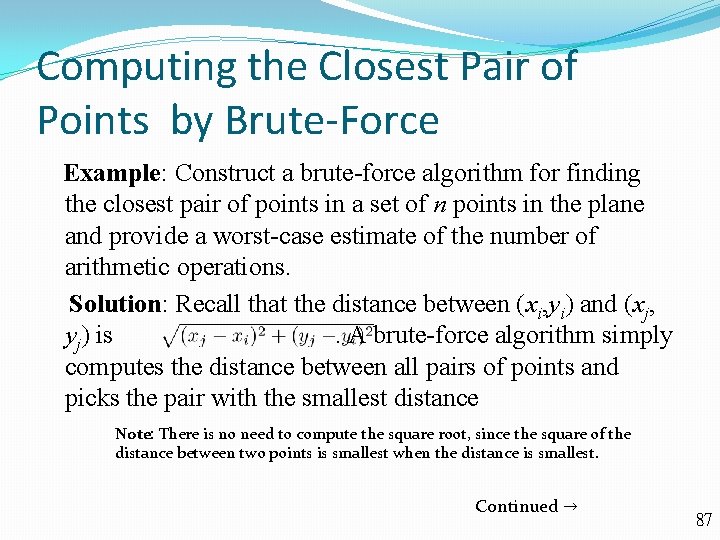
Computing the Closest Pair of Points by Brute-Force Example: Construct a brute-force algorithm for finding the closest pair of points in a set of n points in the plane and provide a worst-case estimate of the number of arithmetic operations. Solution: Recall that the distance between (xi, yi) and (xj, yj) is. A brute-force algorithm simply computes the distance between all pairs of points and picks the pair with the smallest distance Note: There is no need to compute the square root, since the square of the distance between two points is smallest when the distance is smallest. Continued → 87

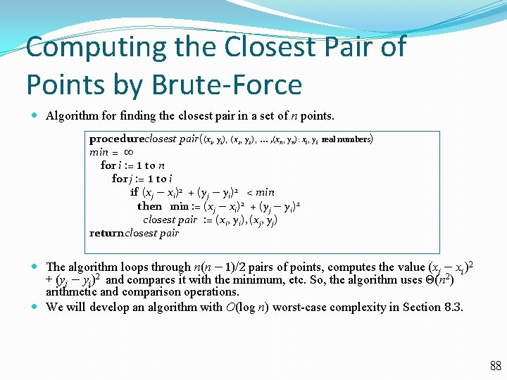
Computing the Closest Pair of Points by Brute-Force Algorithm for finding the closest pair in a set of n points. procedureclosest pair((x 1, y 1), (x 2, y 2), … , (xn, yn): xi, yi min = ∞ for i : = 1 to n for j : = 1 to i if (xj − xi)2 + (yj − yi)2 < min then min : = (xj − xi)2 + (yj − yi)2 closest pair : = (xi, yi), (xj, yj) return closest pair real numbers) The algorithm loops through n(n − 1)/2 pairs of points, computes the value (xj − xi)2 + (yj − yi)2 and compares it with the minimum, etc. So, the algorithm uses Θ(n 2) arithmetic and comparison operations. We will develop an algorithm with O(log n) worst-case complexity in Section 8. 3. 88

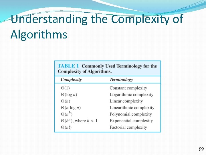
Understanding the Complexity of Algorithms 89

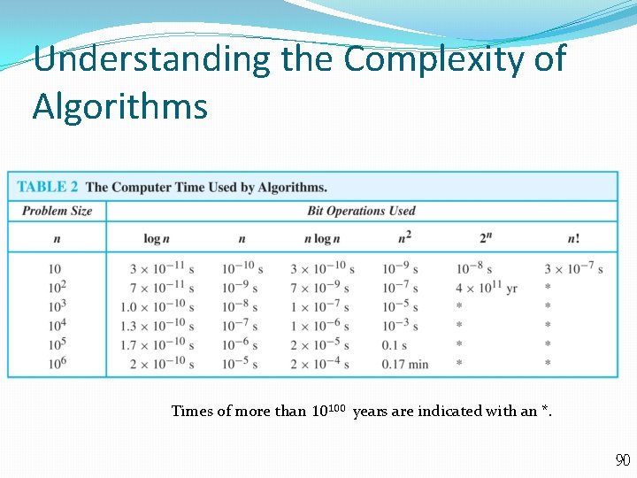
Understanding the Complexity of Algorithms Times of more than 10100 years are indicated with an *. 90

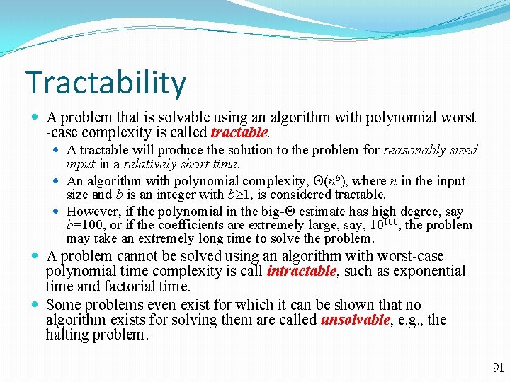
Tractability A problem that is solvable using an algorithm with polynomial worst -case complexity is called tractable. A tractable will produce the solution to the problem for reasonably sized input in a relatively short time. An algorithm with polynomial complexity, (nb), where n in the input size and b is an integer with b 1, is considered tractable. However, if the polynomial in the big- estimate has high degree, say b=100, or if the coefficients are extremely large, say, 10100, the problem may take an extremely long time to solve the problem. A problem cannot be solved using an algorithm with worst-case polynomial time complexity is call intractable, such as exponential time and factorial time. Some problems even exist for which it can be shown that no algorithm exists for solving them are called unsolvable, e. g. , the halting problem. 91

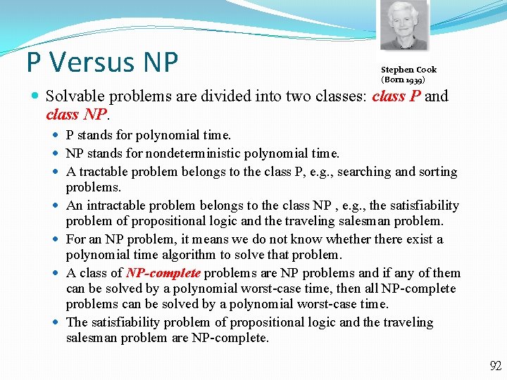
P Versus NP Stephen Cook (Born 1939) Solvable problems are divided into two classes: class P and class NP. P stands for polynomial time. NP stands for nondeterministic polynomial time. A tractable problem belongs to the class P, e. g. , searching and sorting problems. An intractable problem belongs to the class NP , e. g. , the satisfiability problem of propositional logic and the traveling salesman problem. For an NP problem, it means we do not know whethere exist a polynomial time algorithm to solve that problem. A class of NP-complete problems are NP problems and if any of them can be solved by a polynomial worst-case time, then all NP-complete problems can be solved by a polynomial worst-case time. The satisfiability problem of propositional logic and the traveling salesman problem are NP-complete. 92