Travels in CSR space adventures with cellular automata

Travels in (C-S-R) space: adventures with cellular automata Presentation ready with acknowledgements to Ric Colasanti (Corvallis) Andrew Askew (Sheffield)

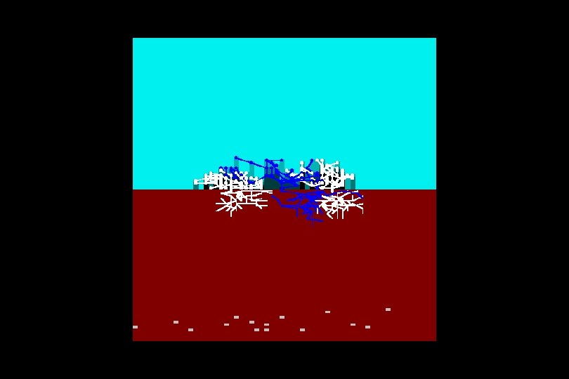
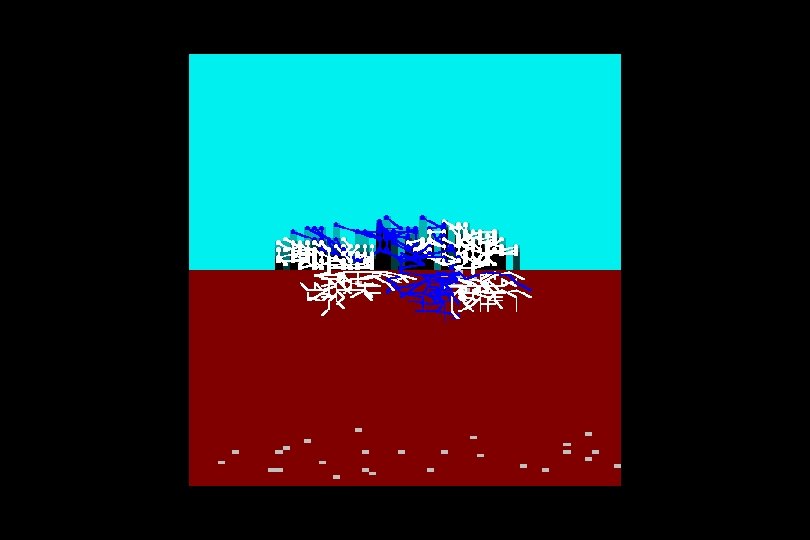
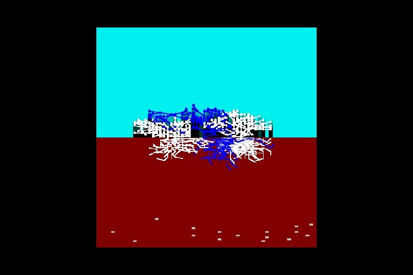
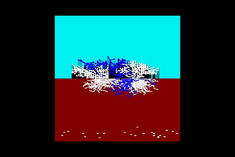
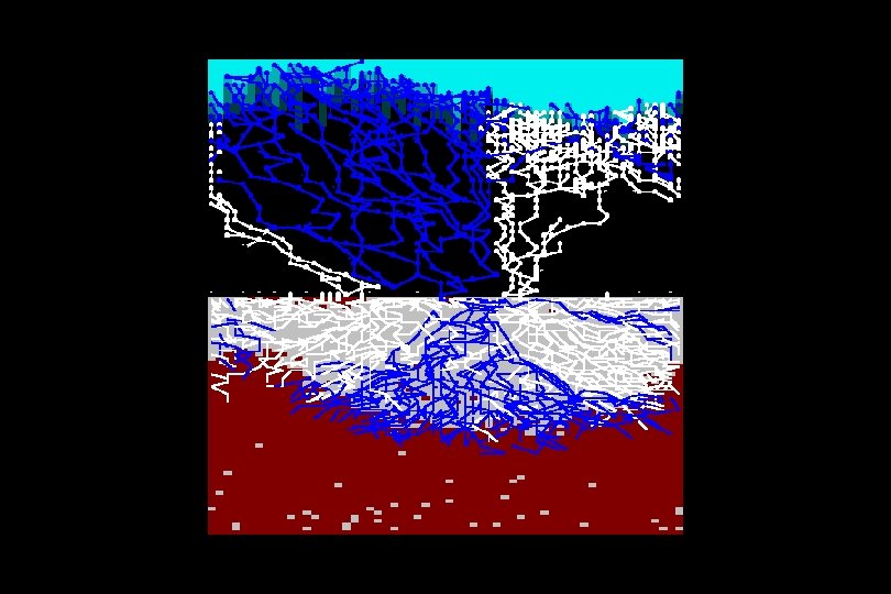
CA in a community of virtual plants Contrasting tones represent patches of

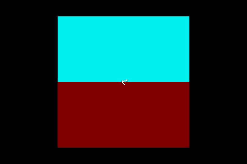
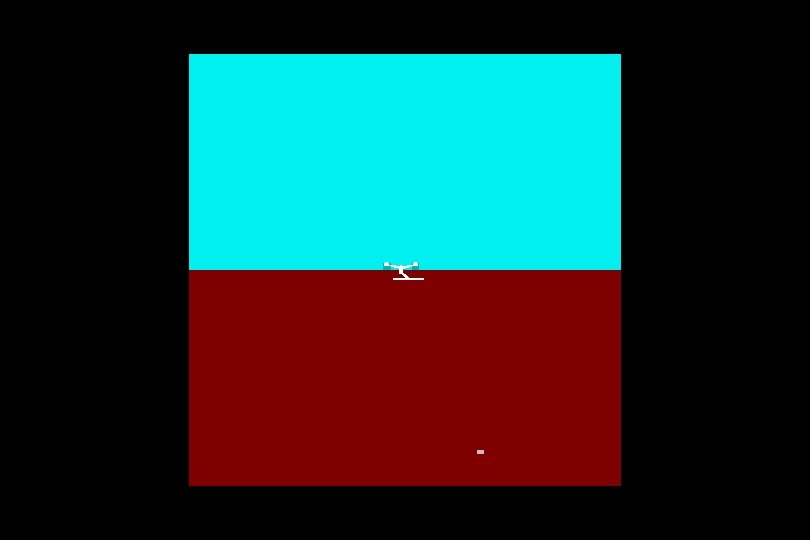
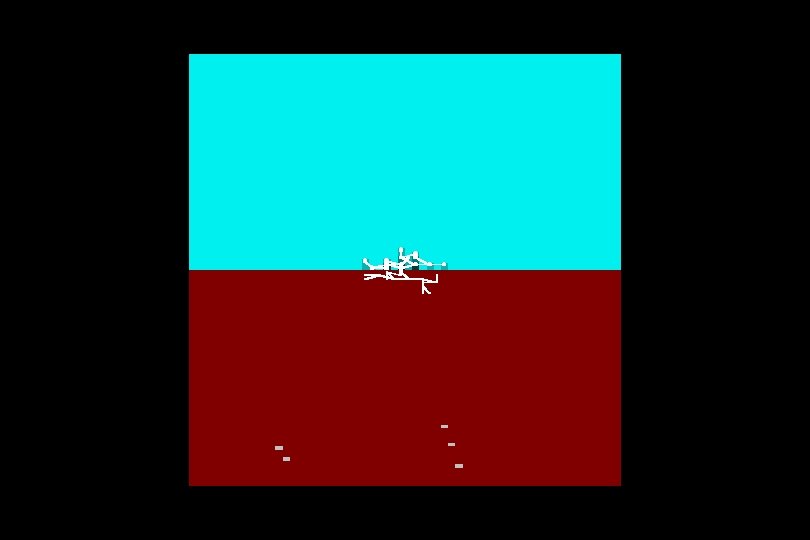
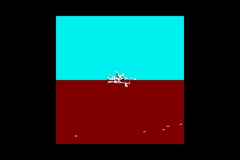
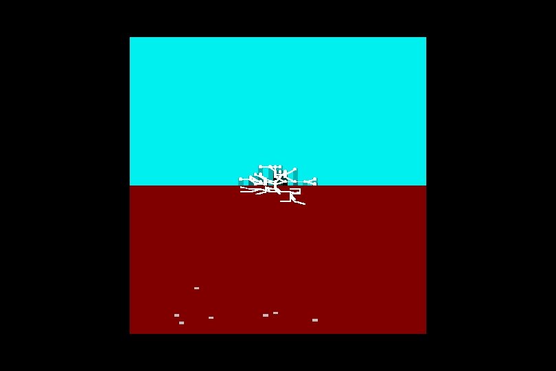
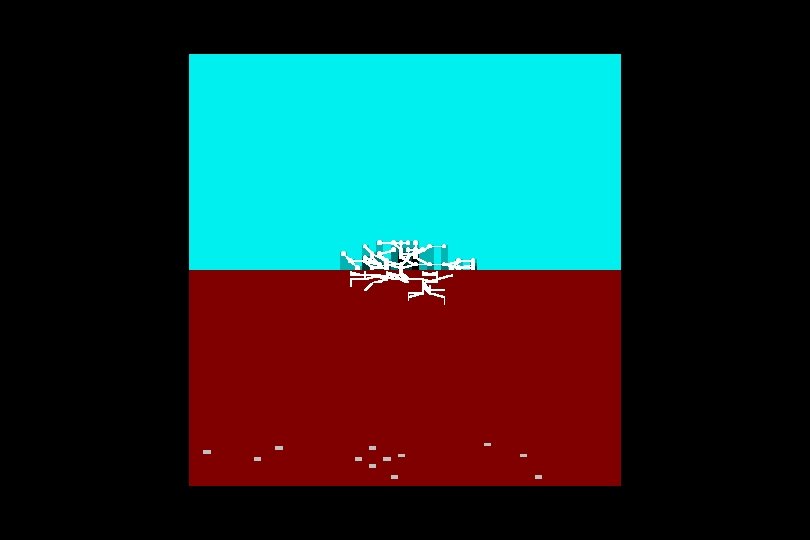
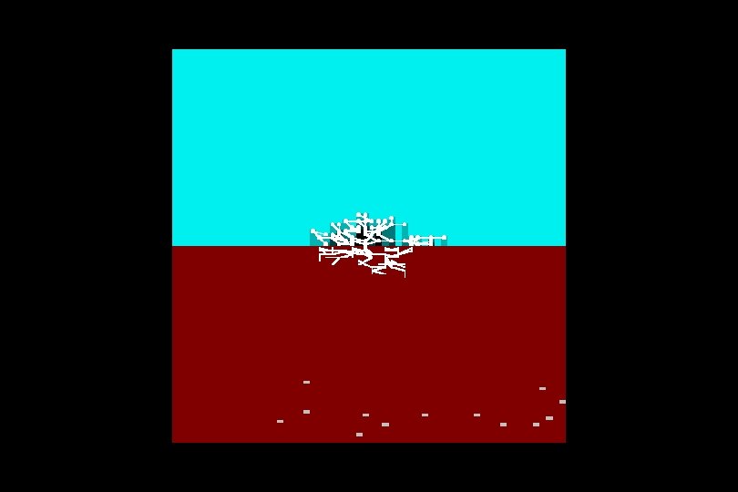
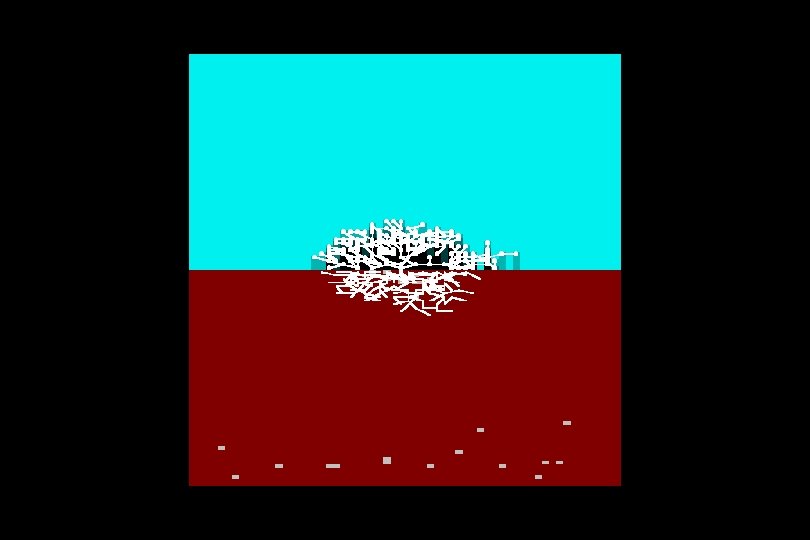
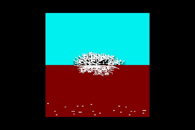
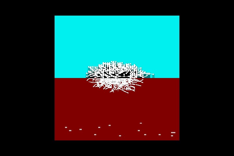
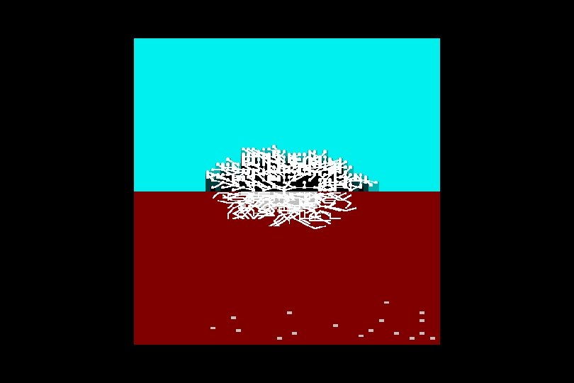
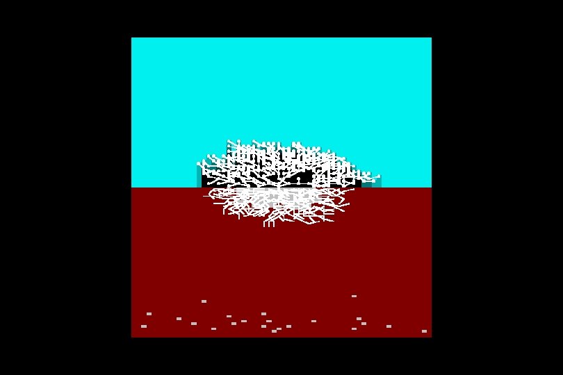
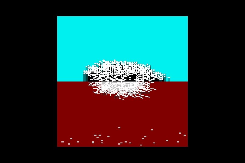
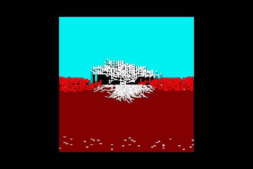
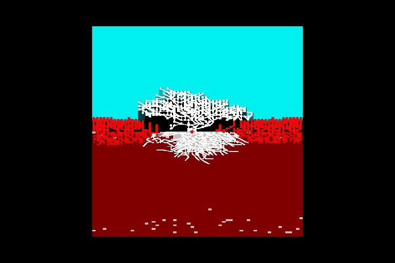
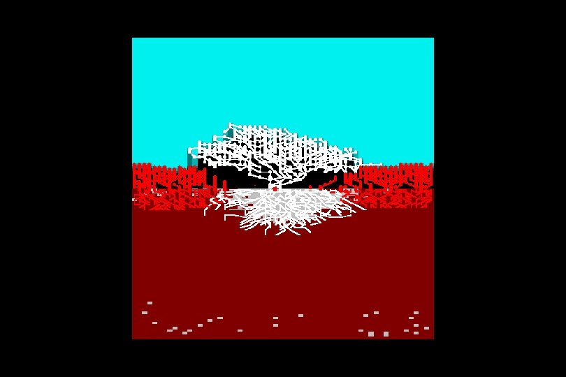
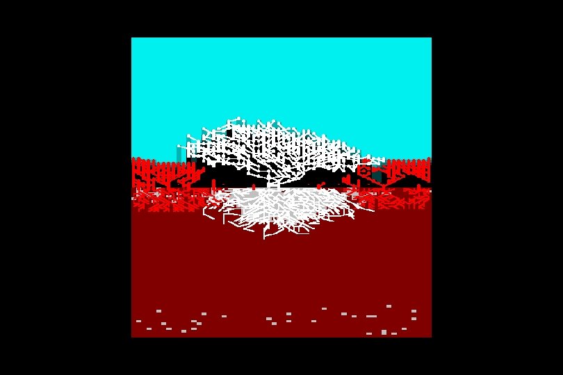
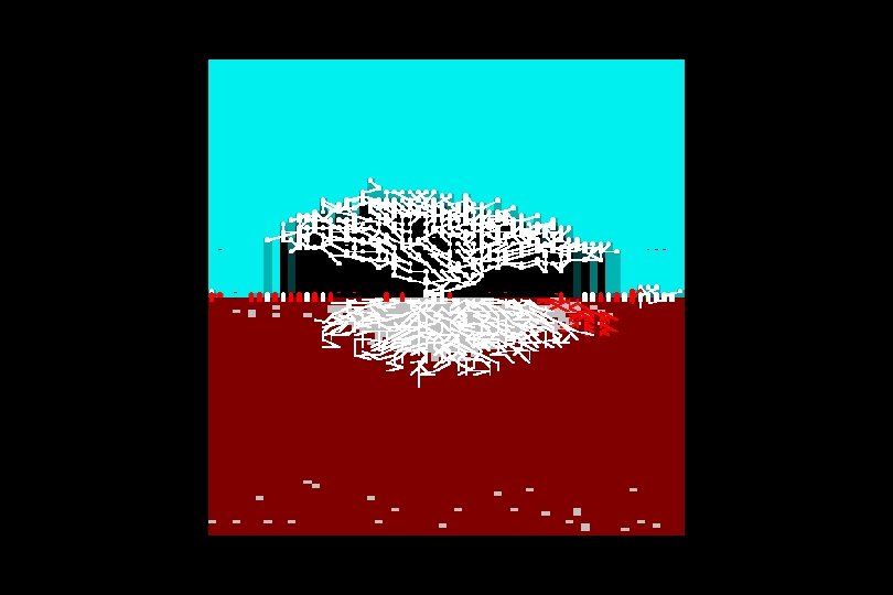
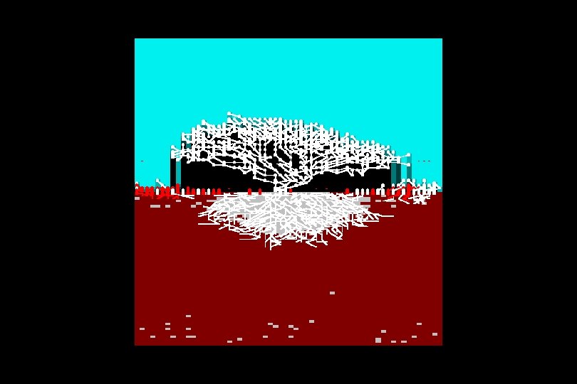
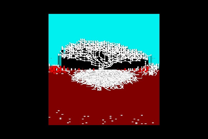
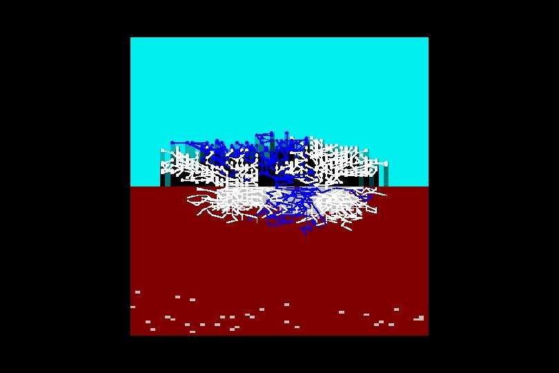
This is a single propagule of a virtual plant It is about to grow in a resource-rich above- and below-ground environment

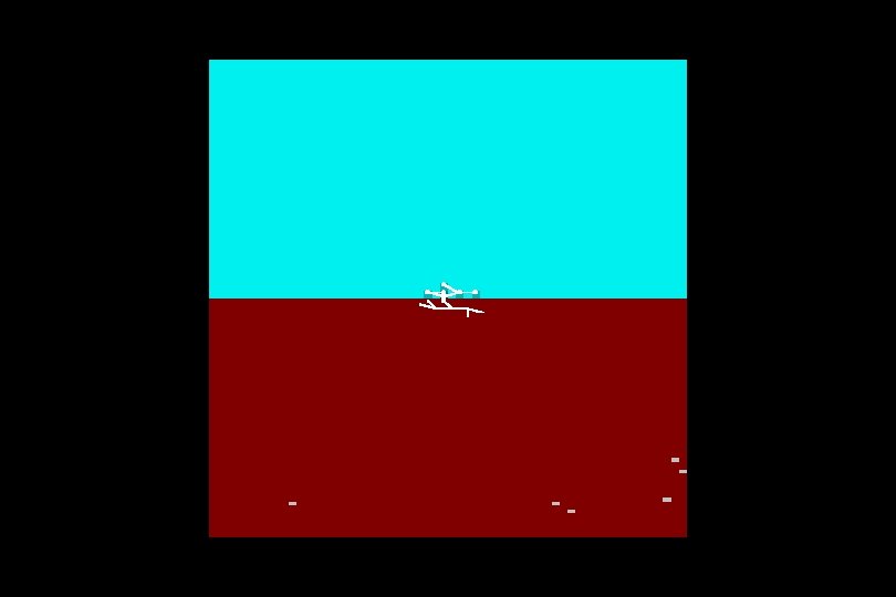
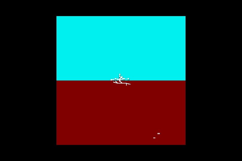
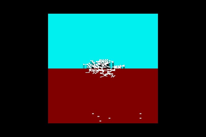
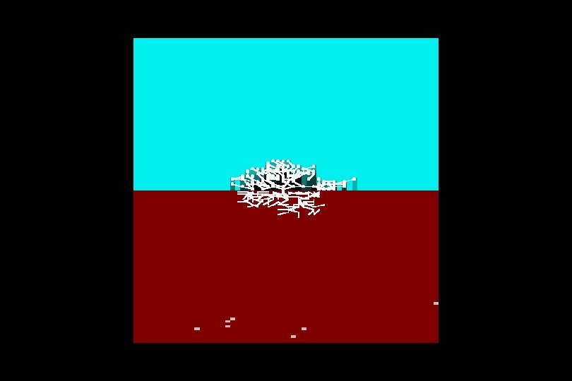
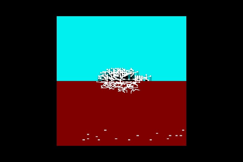
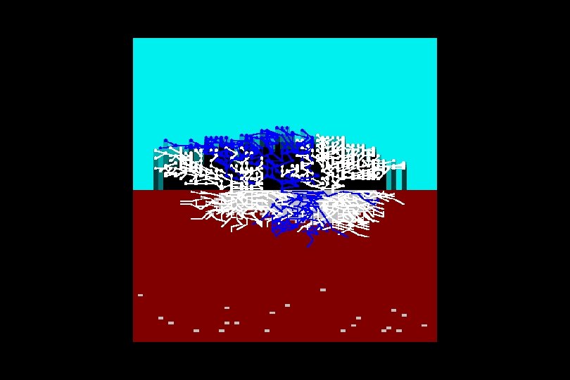
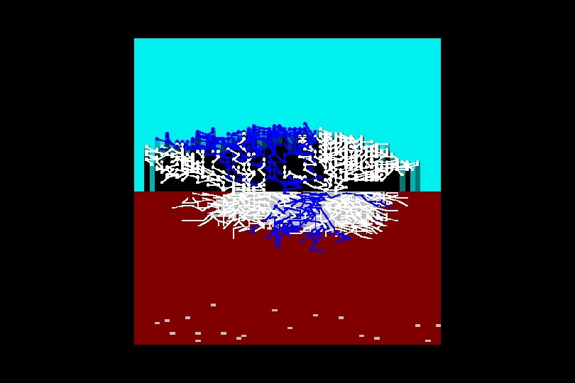
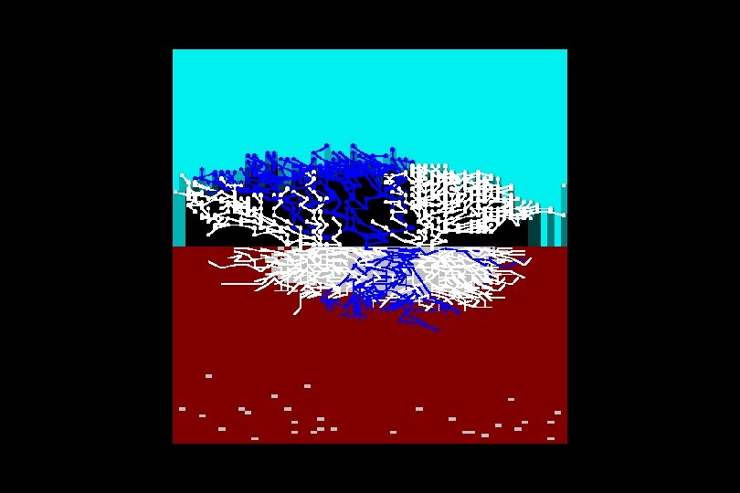
The plant has produced abundant growth aboveand below-ground and zones of resource depletion have appeared

Above-ground binary tree ( = shoot system) Each plant is built-up like this A branching module Above-ground array Above-ground binary tree base module Below-ground array Below-ground binary tree base module This is only a diagram, not a painting ! An end module Below-ground binary tree ( = root system)

The end-modules capture resources: Light and carbon dioxide from aboveground Water and nutrients from belowground The branching modules (parent or offspring) can pass resources to any adjoining modules In this way whole plants can grow

The virtual plants interact with their environment (and with their neighbours) just like real ones do They possess most of the properties of real individuals and populations For example …

Size Time Partitioning between root and shoot S-shaped growth curves Allometric coefficient Individual size Foraging towards resources Below-ground resource Functional equilibria Selfthinning line Population density Self-thinning in crowded populations

All of these plants have the same specification (modular rulebase) And this specification can easily be changed if we want the plants to behave differently… For example, we can recreate J P Grime’s system of C-S-R plant functional types But what is that exactly?

‘ The external factors which limit the amount of living and dead plant material present in any habitat may be classified into two categories ’ Opening sentence from J P Grime’s 1979 book Plant Strategies and Vegetation Processes

Category 1: Stress Phenomena which restrict plant production e. g. shortages of light, water, mineral nutrients, or non-optimal temperature

Category 2: Disturbance Phenomena which destroy plant production e. g. herbivory, pathogenicity, trampling, mowing, ploughing, wind damage, frosting, droughting, soil erosion, burning

Habitats may experience stress and disturbance to any degree and in any combination Stress Disturbance

Low or moderate combinations of stress and disturbance can support vegetation … Stress Disturbance … but extreme combinations of stress and disturbance cannot

There are other ways of describing stress and disturbance Stress Habitat productivity (= resource level) Disturbance Habitat duration

In the domain where vegetation is possible … S Stress-tolerator where S is high but D is low Stress Competitor where both S and D are low C R Disturbance Ruderal where S is low but D is high … plant life has evolved different strategies for dealing with the different combinations

S So this is ‘C-S -R space’ … C R … and these are the ‘habitats’ where no plant life occurs at all

To navigate in C-S-R space we bend the universe a little … S C R

S C R

S C R

S C R

S C R

S C R

S C R

C R S

C S R

C S R

C R S

C R S

C R S

… and recognize an intermediate type C CSR R S

… with further intermediates here C CR R CS CSR SR S

… and yet more intermediates here CR R C CS CSR SR S

So, how does all this relate to real vegetation? The high dimensionality of real plant life is reduced to plant functional types “ There are many more actors on the stage than roles that can be played ”

And what does that mean, exactly? Functional types provide a continuous view of vegetation when relative abundances, and even identities, of constituent species are in flux Tools that allocate C-S-R type to species, and C-S-R position to whole communities, can link separate vegetation into one conceptual framework Then effects of environment or management on biodiversity, vulnerability and stability can be evaluated on a common basis

We can recreate C-S-R plant functional types within the selfassembling model … … if we change the rulebases controlling morphology, physiology and reproductive behaviour …

With three levels possible in each of three traits, 27 simple functional types could be constructed However, we model only 7 types; the other 20 would include Darwinian Demons that do not respect evolutionary tradeoffs

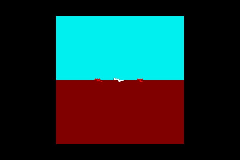
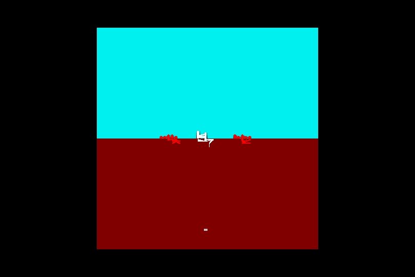
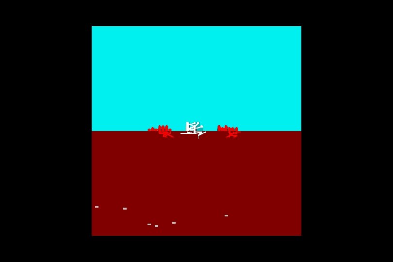
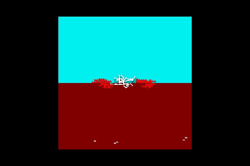
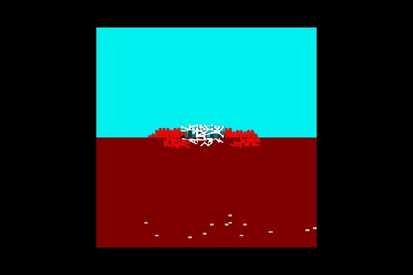
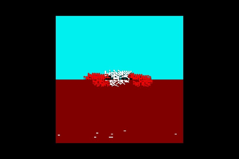
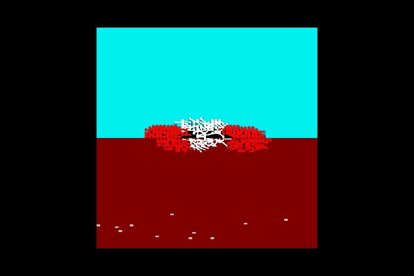
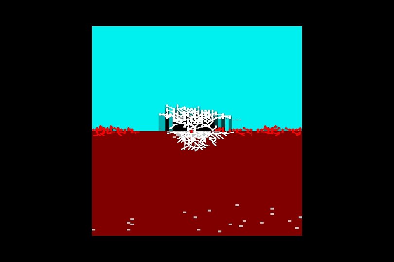
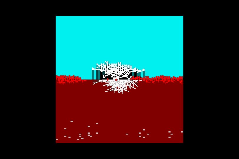
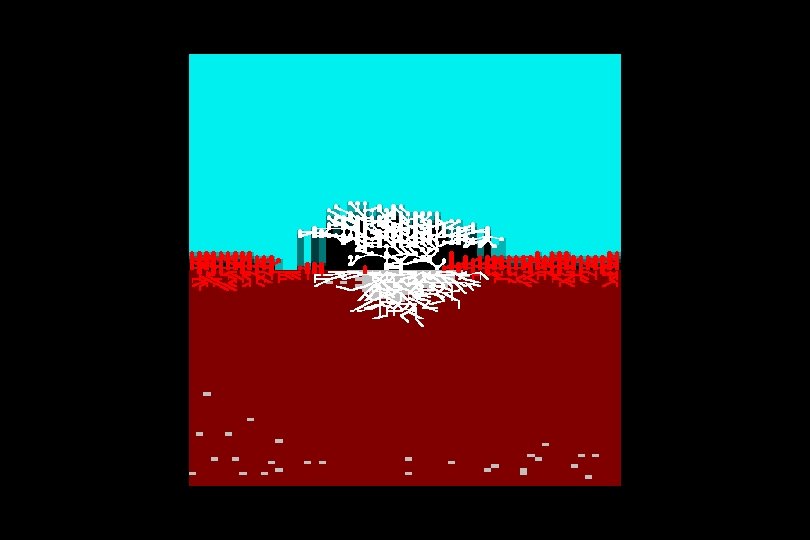
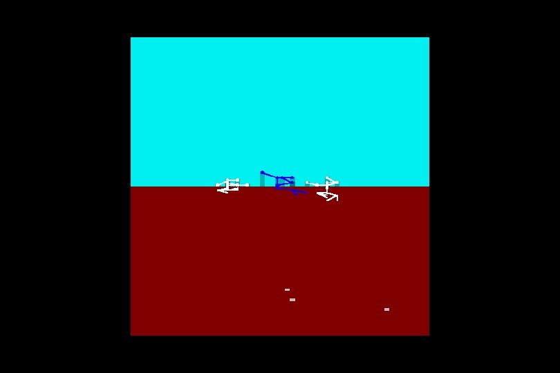
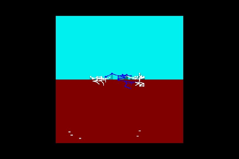
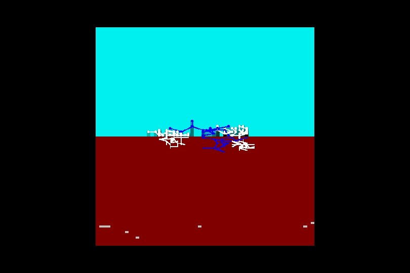
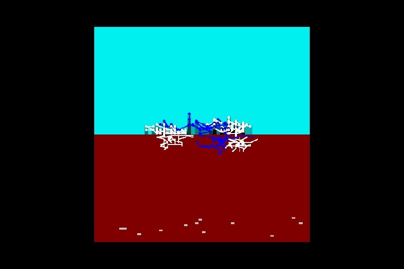
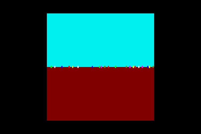
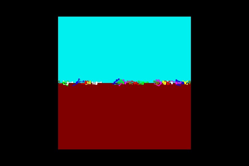
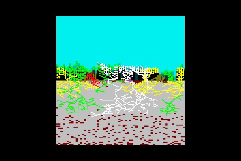
Let’s see some competition between different types of plant Initially we will use only two types …

Small size, rapid growth and fast reproduction Medium size, moderately fast in growth and reproduction

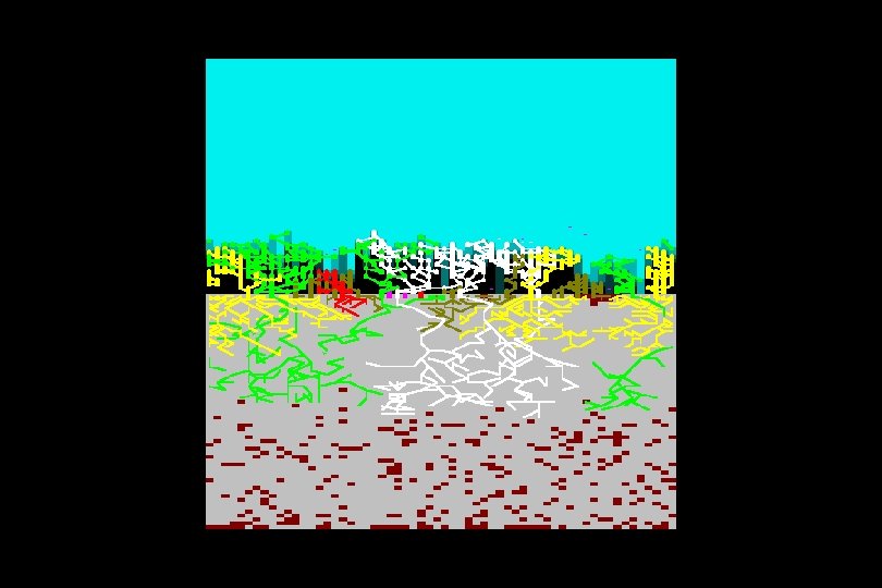
(Red enters its 2 nd generation)

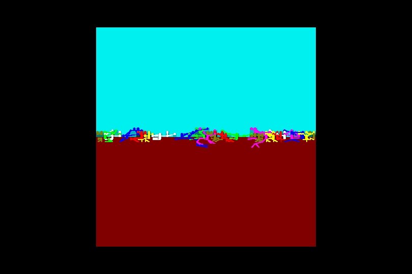
White has won !

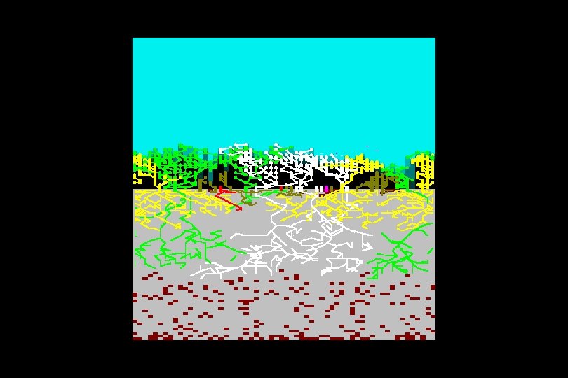
Now let’s see if white always wins This time, the opposition is rather different …

Medium size, moderately fast in growth and reproduction Large size, very fast growing, slow reproductio n

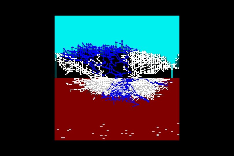
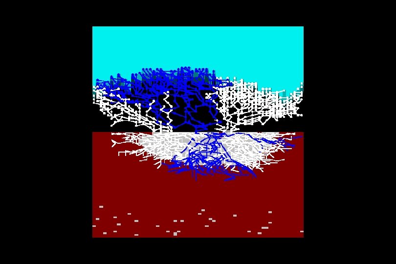
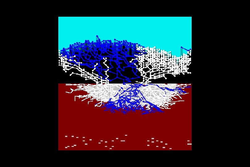
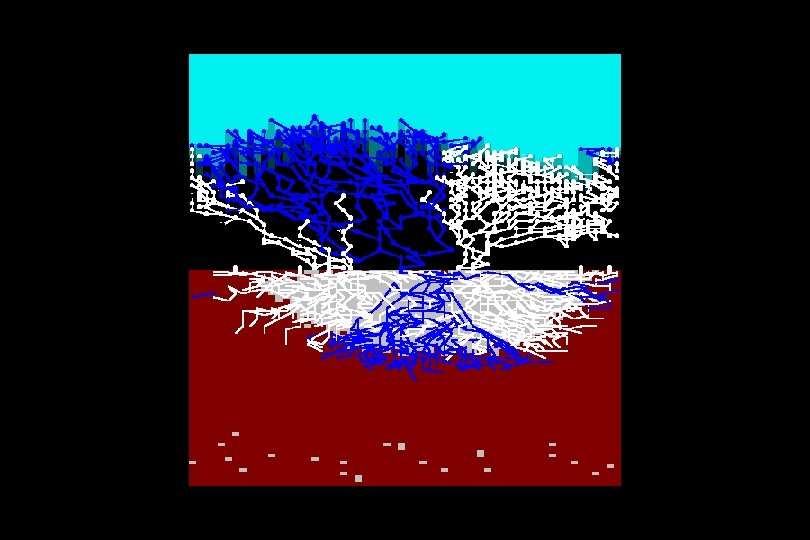
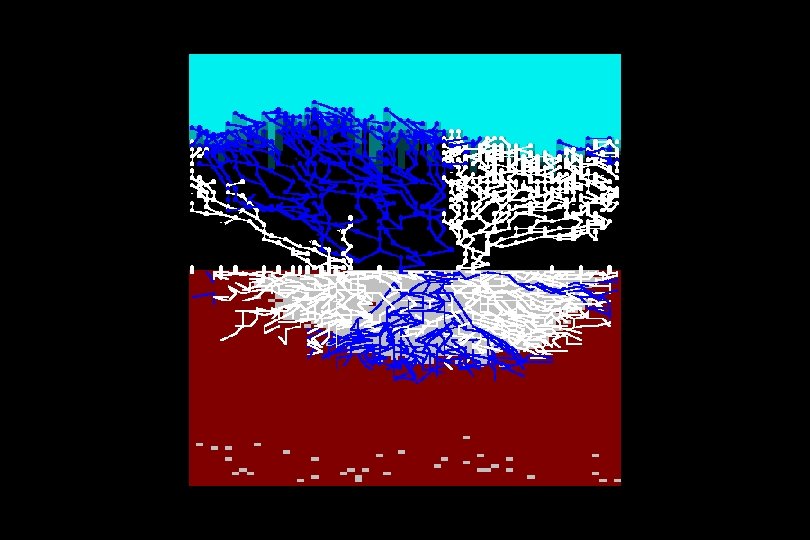
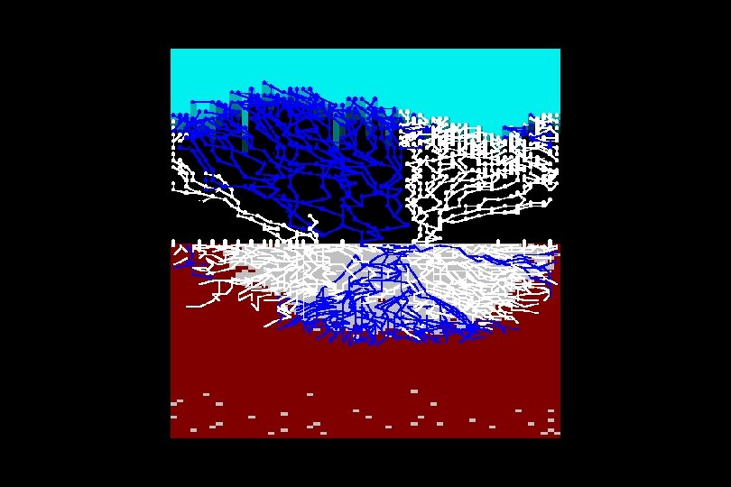
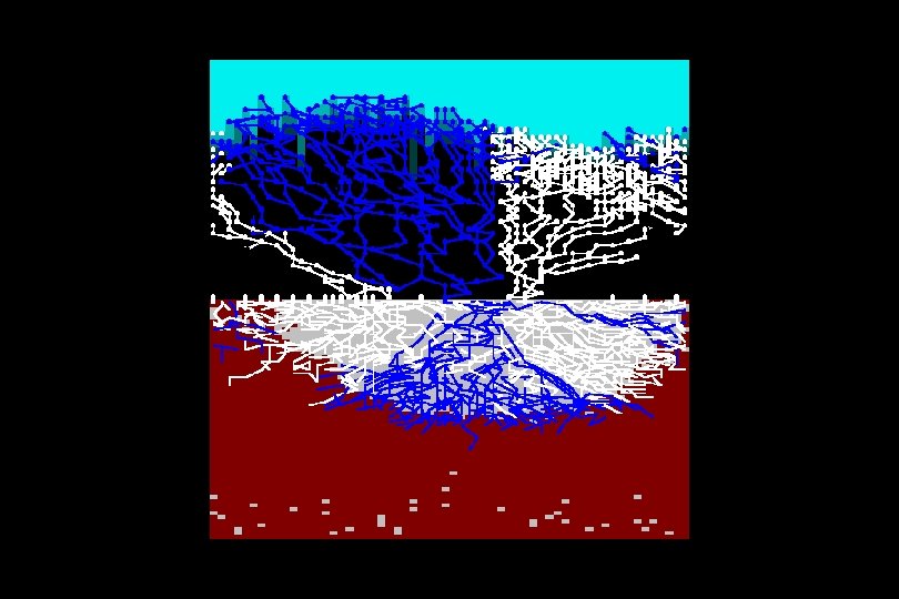
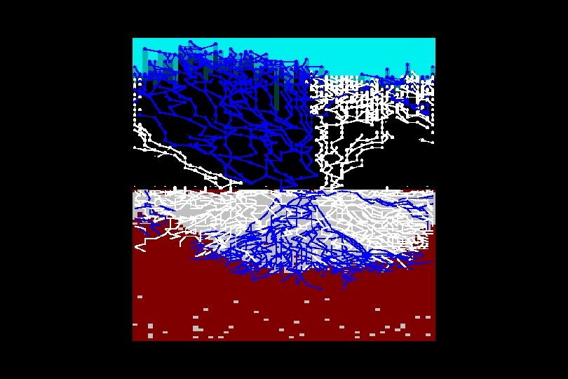
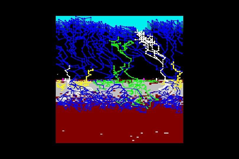
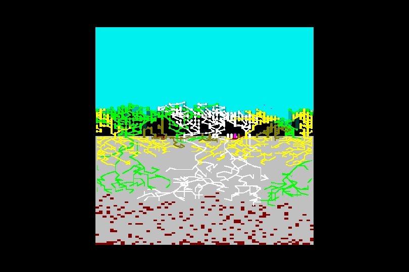
The huge blue type has outcompeted both of the white plants, both above- and belowground And the simulation has run out of space …

So competition can be demonstrated realistically … … but most real communities involve more than two types of plant

We need seven functional types to cover the entire range of variation shown by herbaceous plant life To a first approximation, these seven types can simulate complex community processes very realistically

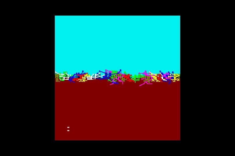
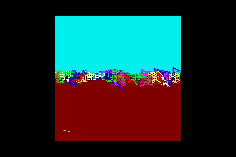
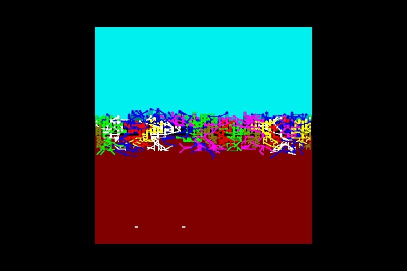
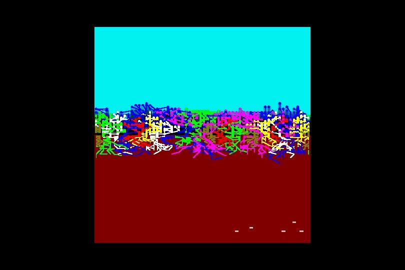
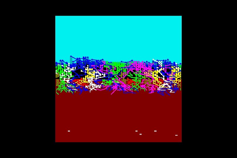
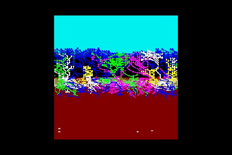
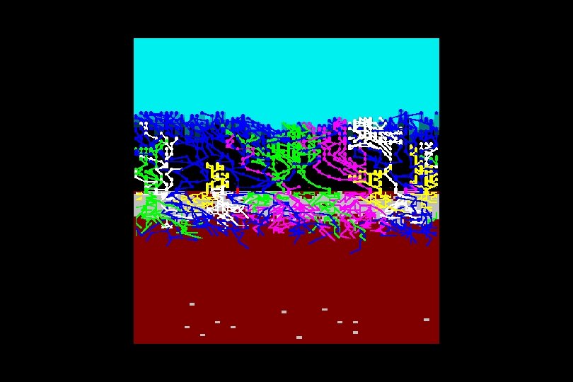
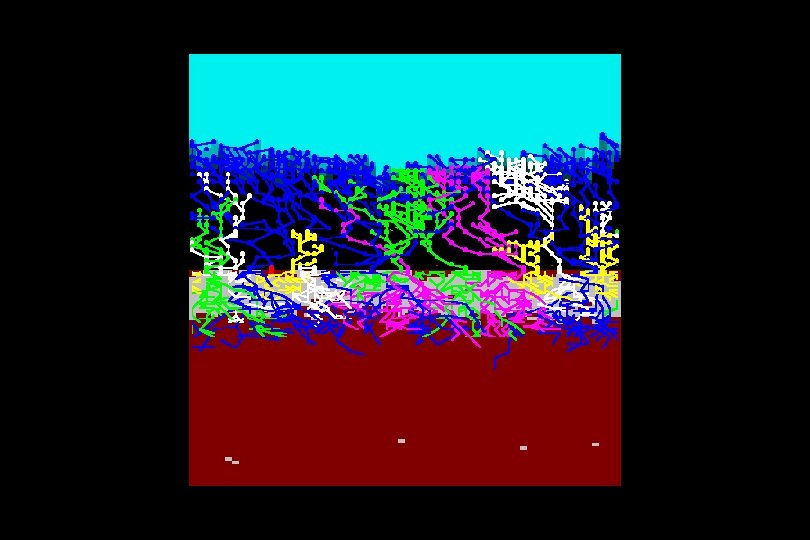
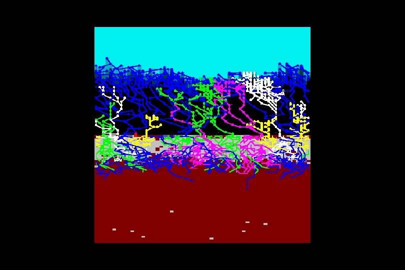
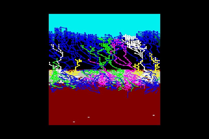
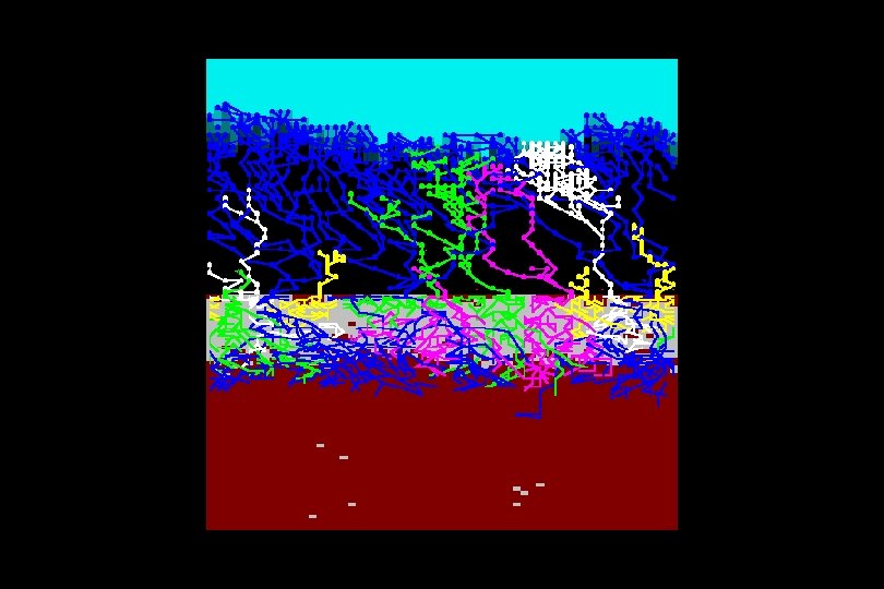
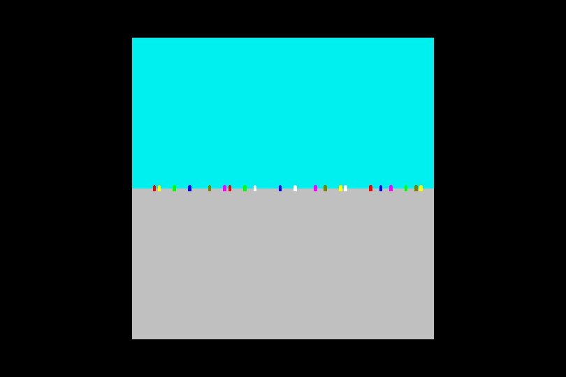
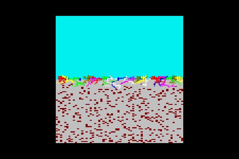
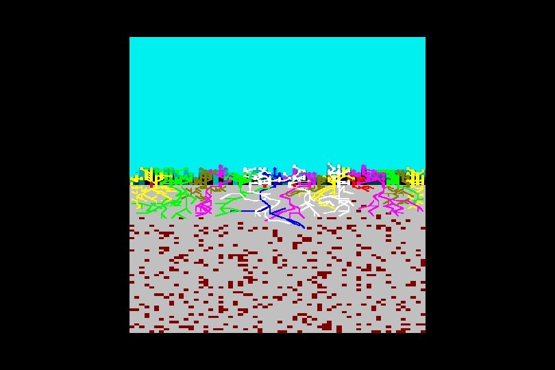
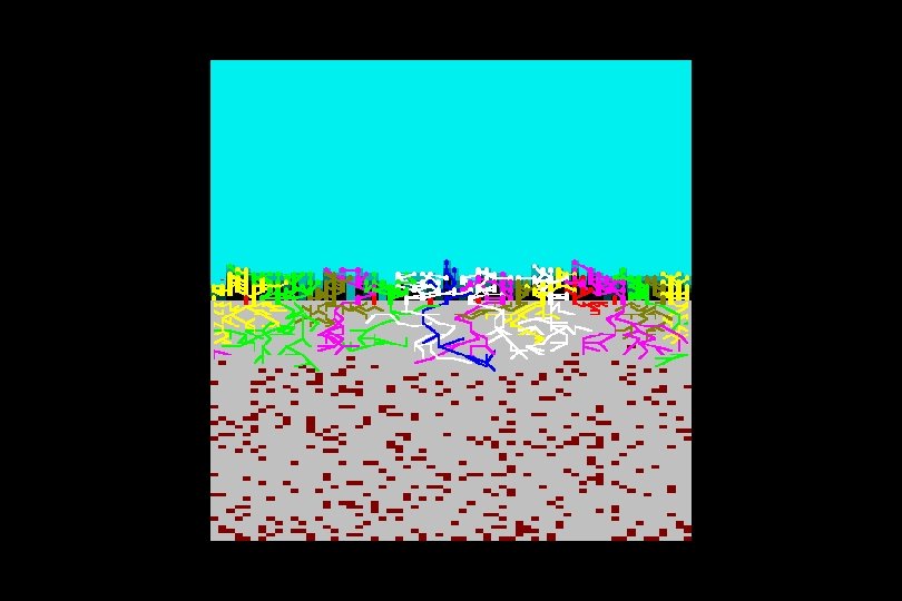
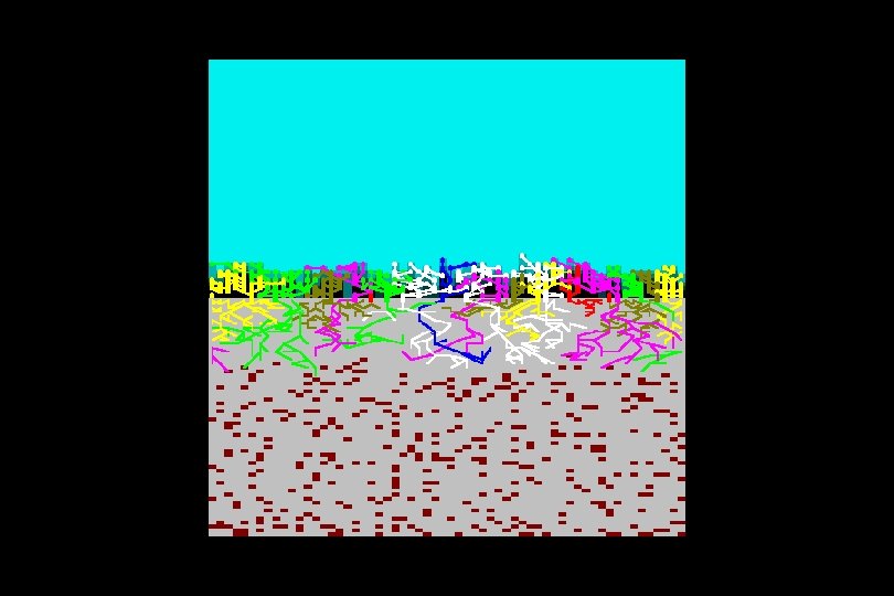
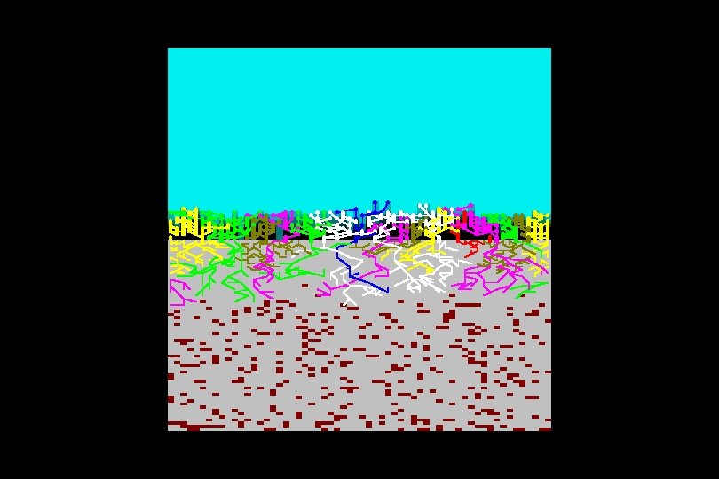
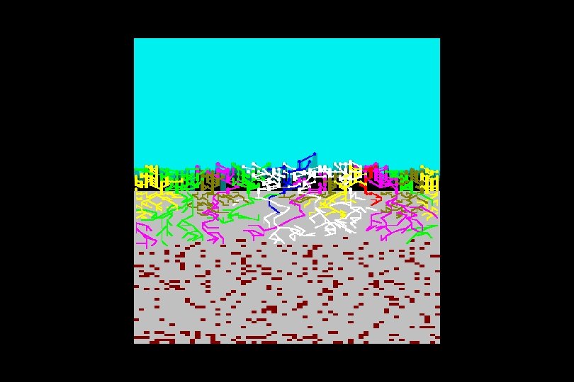
For example, an equal mixture of all seven types can be grown together … … in an environment which has high levels of resource, both above- and below-ground

The blue type has eliminated almost everything except white and green types And the simulation has almost run out of space again …

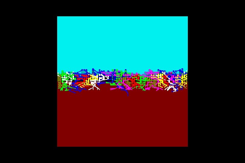
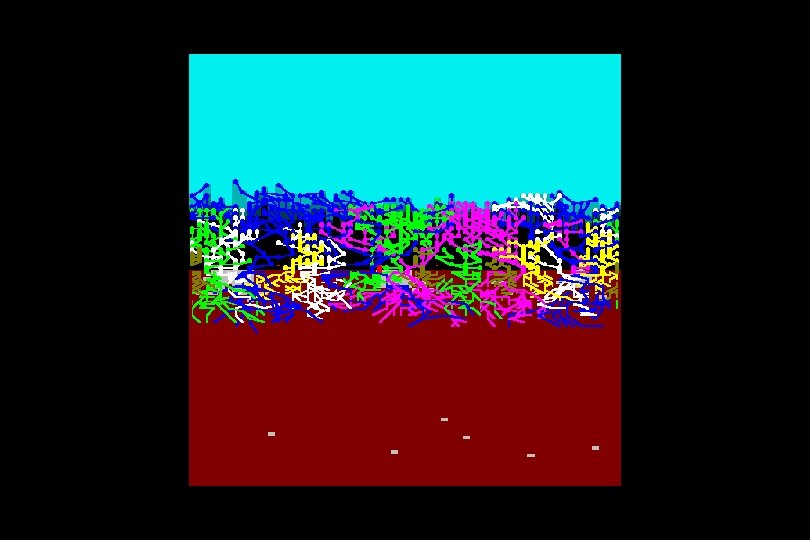
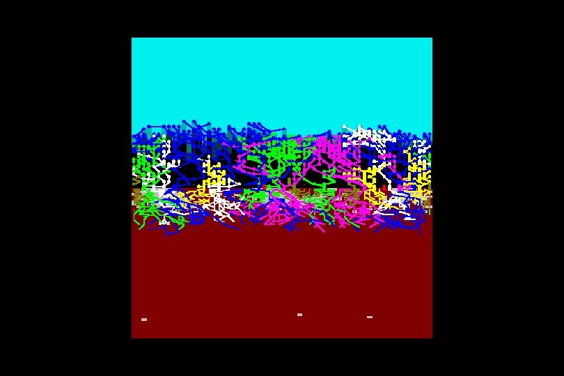
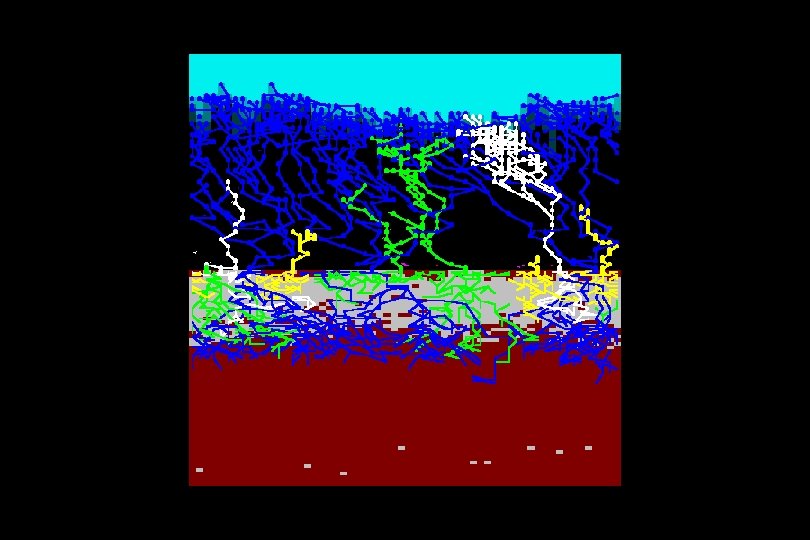
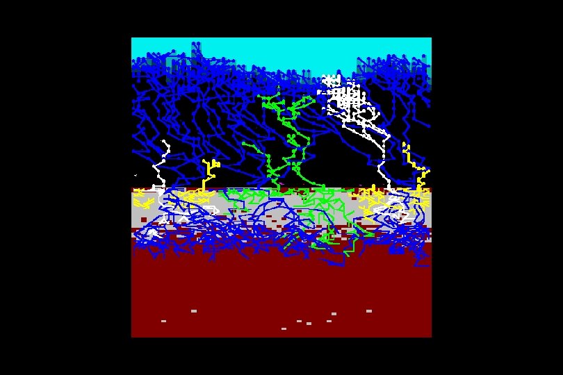
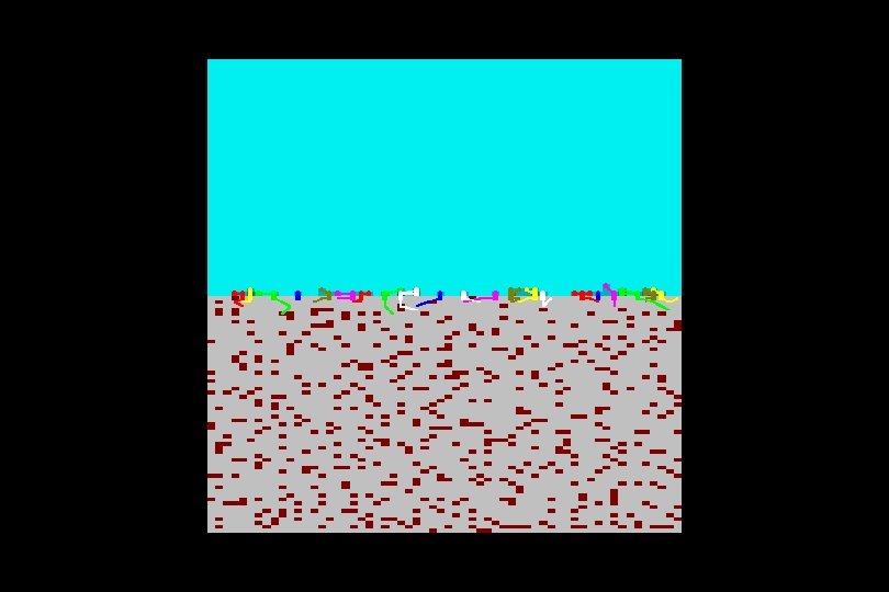
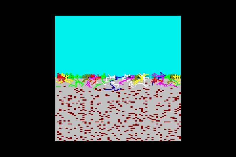
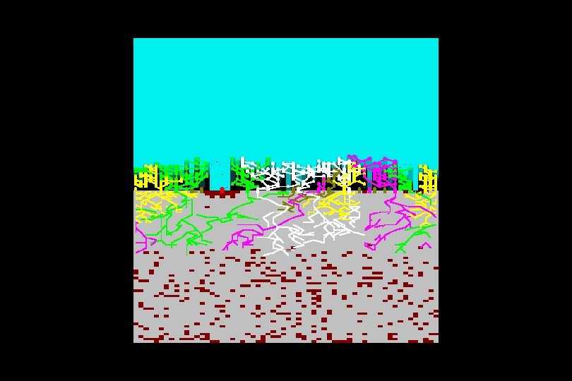
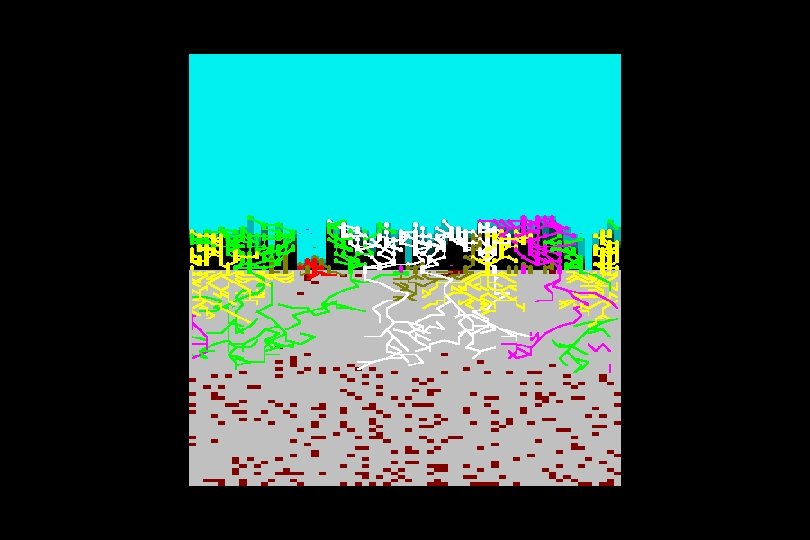
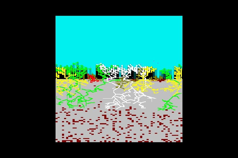
Now let’s grow the equal mixture of all seven types again … … but this time the environment has low levels of mineral nutrient resource (as indicated by the many grey cells)

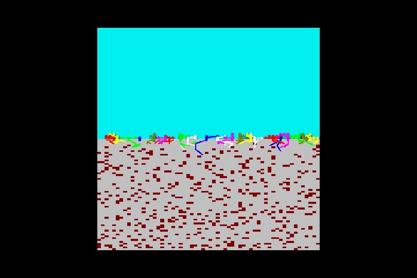
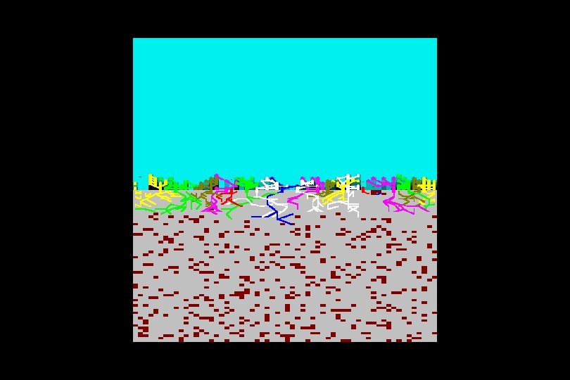
(a gap has appeared here)

(red tries to colonize)

(but is unsuccessful)

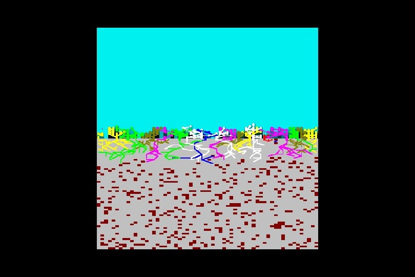
White, green and yellow finally predominate … … blue is nowhere to be seen … … and total biomass is much reduced

Environmental gradients can be simulated by increasing resource levels in steps Whittaker-type niches then appear for contrasting plant types within these gradients

(types)

Let’s grow the equal mixture of all seven types again … … but this time under an environmental gradient of increasing mineral nutrient resource

Greatest biodiversity is at intermediate stress

Remember that environmental disturbance was defined as ‘removal of biomass after it has been created’ Trampling is therefore a disturbance It can be simulated by removing shoot material from certain sizes of patch at certain intervals of time and in a certain number of places

So we grow the equal mixture of all seven types again … … under an environmental gradient of increasing ‘trampling’ disturbance

Greatest biodiversity is at intermediate disturbance … … but the final number of types is low

Environmental stress and disturbance can, of course, be applied together … … and this can be done in all forms and combinations

So, again we grow the equal mixture of all seven types … … but in all factorial combinations of seven levels of stress and seven levels of disturbance

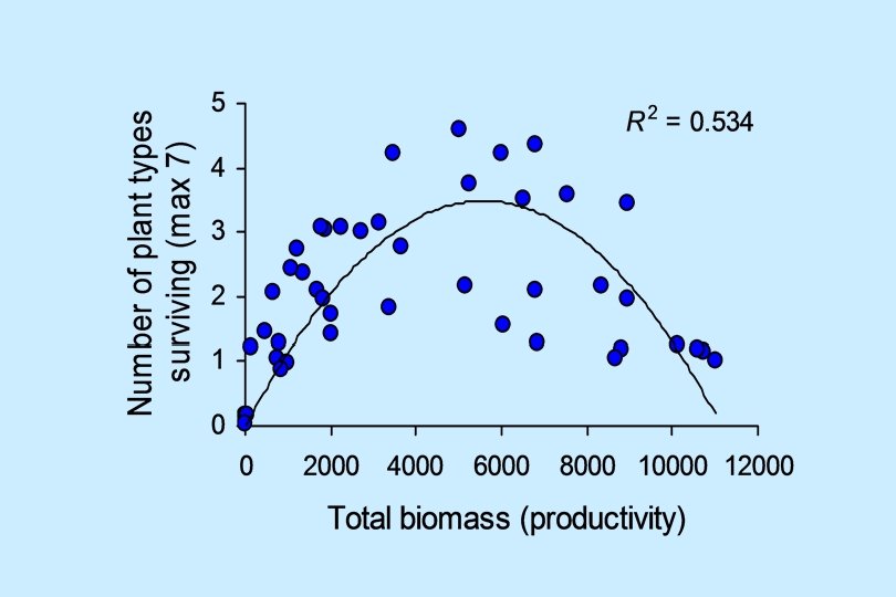
Greatest biodiversity is at intermediate productivity

The biomass-driven ‘humpbacked’ relationship is one of the highest-level properties that real plant communities possess Yet it emerges from the model solely because of the resource-capturing activity of modules in the selfassembling plants

These are all real experiments with virtual plants … and the plant, population and community processes all emerge from the one modular rulebase We can now ‘plant’ whole communities of any kind and subject them to different environments or management regimes Then we can look at topics such as biodiversity, vulnerability, resistance, resilience, stability, habitat / community heterogeneity, etc.

And as the modular rulebase is simply a string of numbers 2314232122133 1 2 controls 3 which how big, how much, how long, how often … (seems familiar? ) … we can modify this 2314232122133 virtual genome 123 wherever we like either accurately 2 3 1 4 2 3 2 1 2 3 123 or inaccurately 2 3 1 4 2 3 2 1 2 2 3 2 1 123 and then follow the downstream consequences of GM

In real experiments with virtual plants … One overnight run on one PC Approx. 100 personyears of growth experiments (not including the transgenic work!) Any takers? http: //www. ex. ac. uk/~rh 2 03/