Cellular Automata 1 Introduction n What are Cellular

Cellular Automata 1

Introduction n What are Cellular Automata? n CA are discrete dynamic systems. n n n CA's are said to be discrete because they operate in finite space and time and with properties that can have only a finite number of states. CA's are said to be dynamic because they exhibit dynamic behaviors. Basic Idea: Simulate complex systems by interaction of cells following easy rules. 2

Introduction n To put it another way: n “Not to describe a complex system with complex equations, but let the complexity emerge by interaction of simple individuals following simple rules. ” 3

Cellular Automata • A CA is a spatial lattice of N cells, each of which is one of k states at time t. • Each cell follows the same simple rule for updating its state. • The cell's state s at time t+1 depends on its own state and the states of some number of neighbouring cells at t. • For one-dimensional CAs, the neighbourhood of a cell consists of the cell itself and r neighbours on either side. Hence, k and r are the parameters of the CA. • CAs are often described as discrete dynamical systems with the capability to model various kinds of natural discrete or continuous dynamical systems 4

History n Original concept of CA is most strongly associated with John von Neumann was interested in the connections between biology and then new study of automata theory. n Stanislaw Ulam suggested that von Neumann use a cellular automata as a framework for researching these connections. 5

History n The original concept of CA can be credited to Ulam, while the early development of the concept is credited to von Neumann. n Although von Neumann made many contributions and developments in CA, they are commonly referred to as “non-von Neumann style”, while the standard model of computation (CPU, globally addressable memory, serial processing) is know as “von Neumann style”. 6

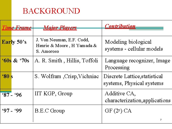
BACKGROUND Time Frame Early 50’s Major Players J. Von Neuman, E. F. Codd, Henrie & Moore , H Yamada & S. Amoroso ‘ 60 s & ‘ 70 s A. R. Smith , Hillis, Toffoli Contribution Modeling biological systems - cellular models Language recognizer, Image Processing ‘ 80 s S. Wolfram , Crisp, Vichniac Discrete Lattice, statistical systems, Physical systems ‘ 87 - ‘ 96 IIT KGP, Group Additive CA, characterization, applications ‘ 97 - ‘ 99 B. E. C Group GF (2 p) CA 7

Why should we study Cellular Automata? n Powerful computation engines. n Discrete dynamical system simulators. n Conceptual vehicle for exploring pattern formation. n Models of fundamental physics. 8

Why should we study Cellular Automata? n Powerful computation engines. n Allow very efficient parallel computation n Discrete dynamical system simulator. n Allow for a systematic investigation of complex phenomena. n Original models of fundamental physics. n Instead of looking at the equations of fundamental physics, consider modelling them with CA. 9

Applications n Simulations n Gas behavior n Forest fire propagation n Urban development n Traffic flow n Air flow n Crystallization process n Alternative to differential equations 10

Components n Cell n Basic element of a CA. n Cells can be thought of as memory elements that store state information. n All cells are updated synchronously according to the transition rules. n Lattice n Spatial web of cells. n Simplest lattice is one dimensional. 11

Behavior n Local interaction leads to global dynamics. n One can think of the behavior of a cellular automata like that of a “wave” at a sports event. n Each person reacts to the state of his neighbors (if they stand, he stands). 12

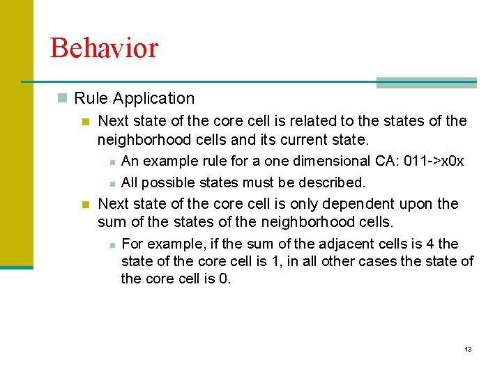
Behavior n Rule Application n Next state of the core cell is related to the states of the neighborhood cells and its current state. n An example rule for a one dimensional CA: 011 ->x 0 x n All possible states must be described. n Next state of the core cell is only dependent upon the sum of the states of the neighborhood cells. n For example, if the sum of the adjacent cells is 4 the state of the core cell is 1, in all other cases the state of the core cell is 0. 13

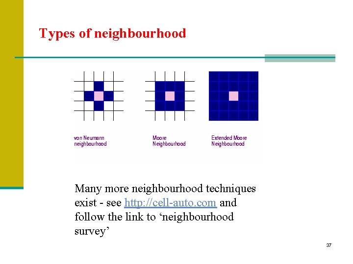
Behavior n Neighborhoods n von Neumann n Moore n Extended Moore n What about border cells? n Common approach is to “wrap” around. 14

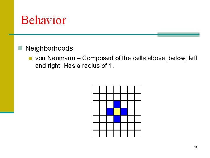
Behavior n Neighborhoods n von Neumann – Composed of the cells above, below, left and right. Has a radius of 1. 15

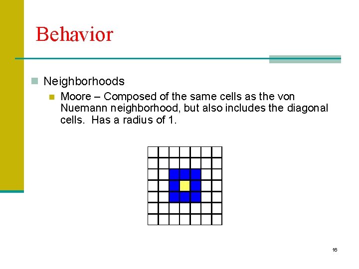
Behavior n Neighborhoods n Moore – Composed of the same cells as the von Nuemann neighborhood, but also includes the diagonal cells. Has a radius of 1. 16

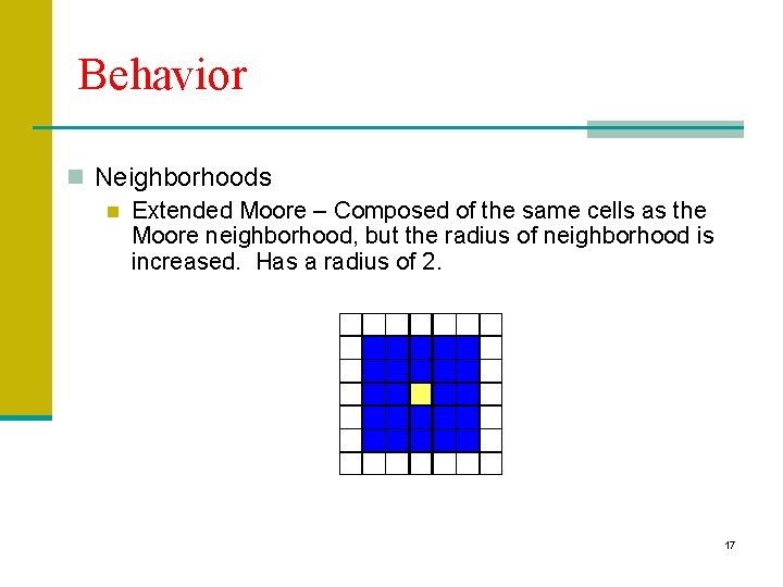
Behavior n Neighborhoods n Extended Moore – Composed of the same cells as the Moore neighborhood, but the radius of neighborhood is increased. Has a radius of 2. 17

Behavior n Rule Systems n Rule systems define the dynamic behavior of the CA. n Even in a simple one dimensional system, there are many different ways to determine the next step. § Could base the next state of the cell off of the sum of the states of your neighbors (Game of Life). § Could modify the scope of the neighborhood, so the resulting neighbors could be local (touching), close (neighbor’s neighbors) or global (anywhere in the system) or possibly use random neighbors. § Could allow the cells to grow and die. 18

Characteristics n Discrete lattice of cells. n Homogeneity – all of the cells of the lattice are equivalent. n Discrete states – each cell takes on one of a finite number of possible discrete states. n Local interactions – each cell interacts only with cells that are in its local neighborhood. 19

Characteristics n Discrete dynamics – at each discrete time unit, each cell updates its current state according to a transition rule taking into account the states of the cells in its neighbourhood. 20

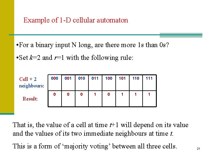
Example of 1 -D cellular automaton • For a binary input N long, are there more 1 s than 0 s? • Set k=2 and r=1 with the following rule: Cell + 2 neighbours: Result: 000 001 010 011 100 101 110 111 0 0 0 1 1 1 That is, the value of a cell at time t+1 will depend on its value and the values of its two immediate neighbours at time t. This is a form of ‘majority voting’ between all three cells. 21

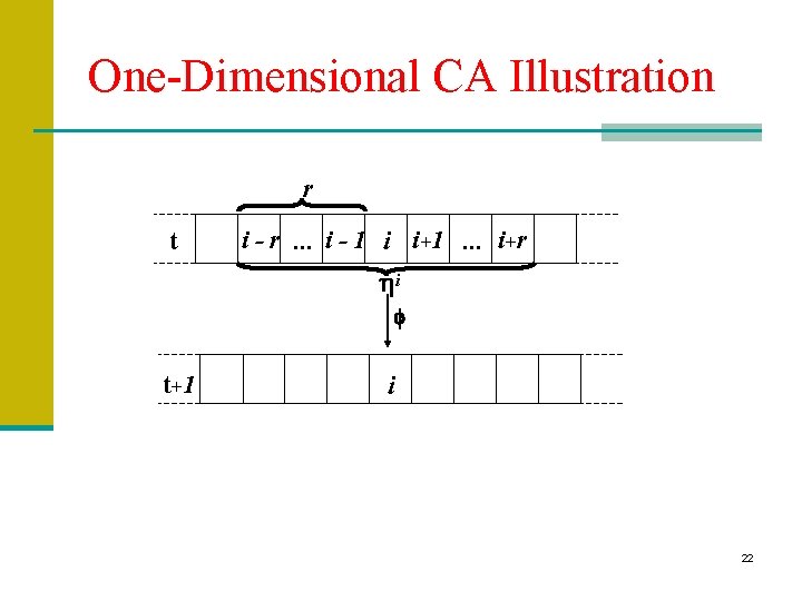
One-Dimensional CA Illustration r t i - r. . . i - 1 i i+1. . . i+r hi f t+ 1 i 22

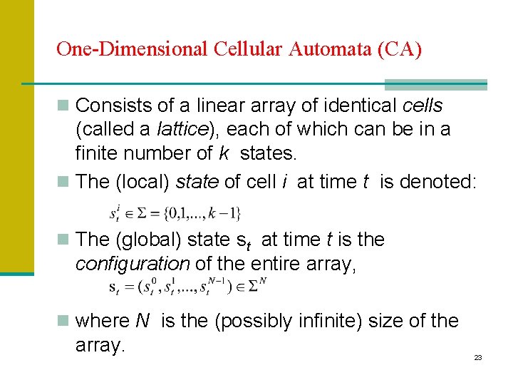
One-Dimensional Cellular Automata (CA) n Consists of a linear array of identical cells (called a lattice), each of which can be in a finite number of k states. n The (local) state of cell i at time t is denoted: n The (global) state st at time t is the configuration of the entire array, n where N is the (possibly infinite) size of the array. 23

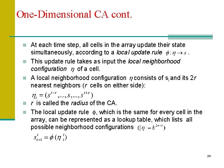
One-Dimensional CA cont. n At each time step, all cells in the array update their state simultaneously, according to a local update rule. n This update rule takes as input the local neighborhood configuration of a cell. n A local neighborhood configuration consists of si and its 2 r nearest neighbors (r cells on either side): n r is called the radius of the CA. n The local update rule , which is the same for every cell in the array, can be represented as a lookup table, which lists all possible neighborhood configurations 24

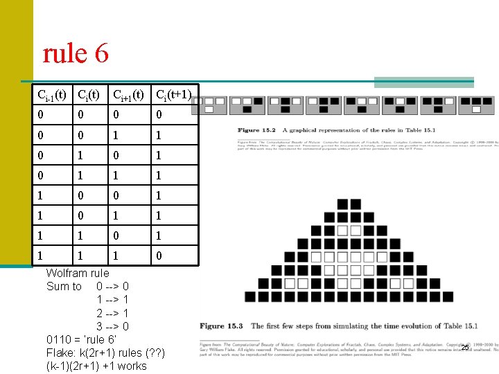
rule 6 Ci-1(t) Ci+1(t) Ci(t+1) 0 0 0 1 1 0 1 0 1 1 0 0 1 1 1 1 0 Wolfram rule Sum to 0 --> 0 1 --> 1 2 --> 1 3 --> 0 0110 = ‘rule 6’ Flake: k(2 r+1) rules (? ? ) (k-1)(2 r+1) +1 works 25

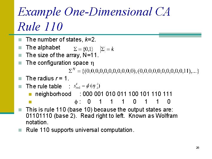
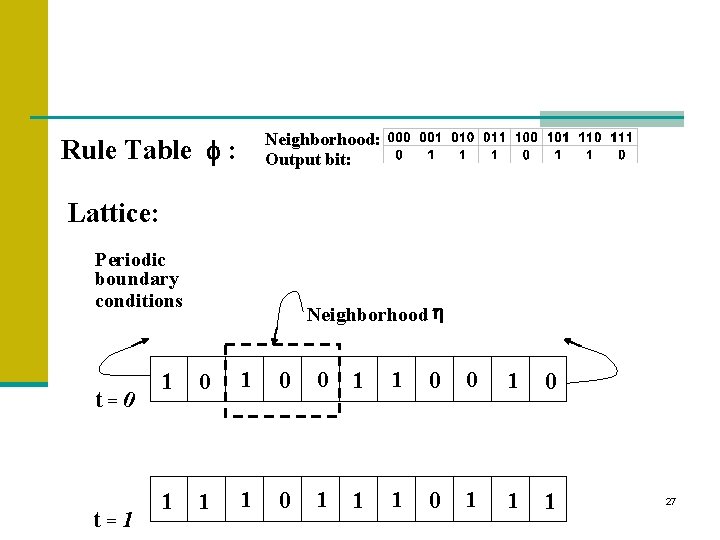
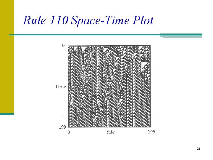
Example One-Dimensional CA Rule 110 n n The number of states, k=2. The alphabet The size of the array, N=11. The configuration space n The radius r = 1. n The rule table : : 000 001 010 011 100 101 110 111 n : 0 1 1 1 0 n This is rule 110 (base 10) because the output states are: 01101110 (base 2). Read right to left. Known as Wolfram notation. n Rule 110 supports universal computation. n neighborhood 26

Neighborhood: Output bit: Rule Table f : Lattice: Periodic boundary conditions t=0 t=1 Neighborhood h 1 0 0 1 1 1 0 1 1 1 27

Rule 110 Space-Time Plot 28

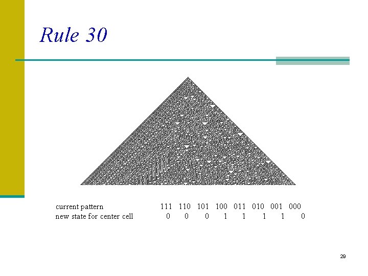
Rule 30 current pattern new state for center cell 111 110 101 100 011 010 001 000 0 1 1 0 29

Comments on Rule 30 n Generates apparent randomness, despite being finite n Wolfram proposed using the central column as a pseudo- random number generator n Passes many tests for randomness, but many inputs produce regular patterns: n All zeroes n 0000111000 repeated infinitely (try separating by 6 1 s) n Used in Mathematica for creating random integers (Wikipedia) 30

Variants n Asynchronous CA n CA rules are typically applied simultaneously across all cells in the lattice. This variant allows the state of the cells to be updated asynchronously. n Probabilistic CA n The deterministic state-transitions are replaced with specifications of the probabilities of the cell -value assignments. 31

Variants n Non-homogenous CA n State transition rules are allowed to vary from cell to cell. n Mobile CA n Some or all lattice sites are free to move about the lattice. n Essentially primitive models of mobile robots. n Used to model some aspects of military engagements. 32

Variants n Structurally Dynamic CA n The topology (the sites and connections among sites) are allowed to evolve. 33

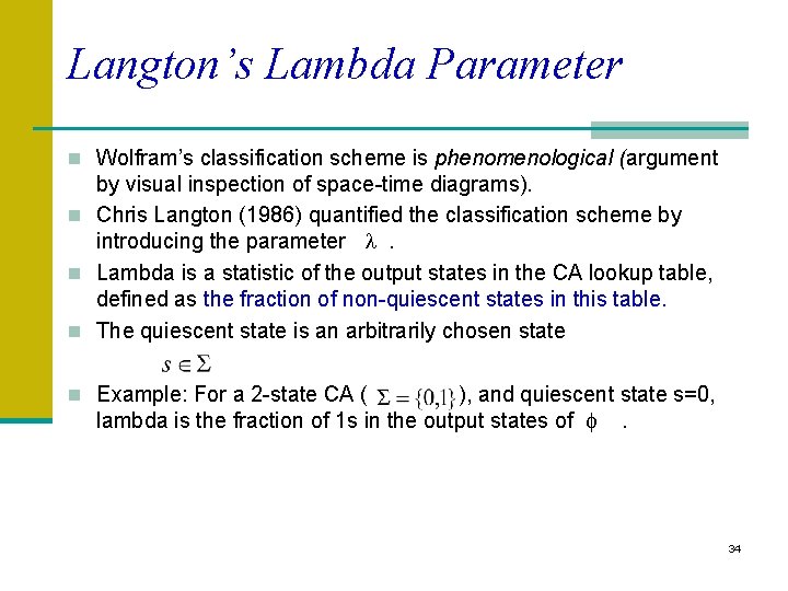
Langton’s Lambda Parameter n Wolfram’s classification scheme is phenomenological (argument by visual inspection of space-time diagrams). n Chris Langton (1986) quantified the classification scheme by introducing the parameter . n Lambda is a statistic of the output states in the CA lookup table, defined as the fraction of non-quiescent states in this table. n The quiescent state is an arbitrarily chosen state n Example: For a 2 -state CA ( ), and quiescent state s=0, lambda is the fraction of 1 s in the output states of . 34

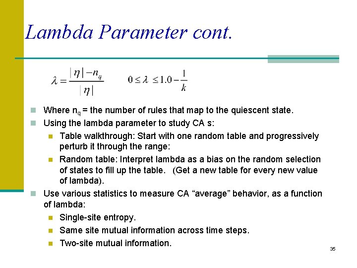
Lambda Parameter cont. n Where nq = the number of rules that map to the quiescent state. n Using the lambda parameter to study CA s: Table walkthrough: Start with one random table and progressively perturb it through the range: n Random table: Interpret lambda as a bias on the random selection of states to fill up the table. (Get a new table for every new value of lambda). n Use various statistics to measure CA “average” behavior, as a function of lambda: n Single-site entropy. n Same site mutual information across time steps. n Two-site mutual information. n 35

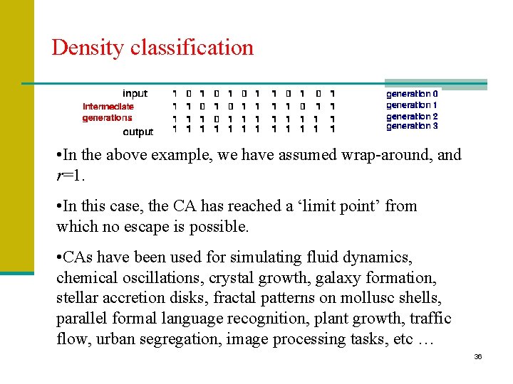
Density classification • In the above example, we have assumed wrap-around, and r=1. • In this case, the CA has reached a ‘limit point’ from which no escape is possible. • CAs have been used for simulating fluid dynamics, chemical oscillations, crystal growth, galaxy formation, stellar accretion disks, fractal patterns on mollusc shells, parallel formal language recognition, plant growth, traffic flow, urban segregation, image processing tasks, etc … 36

Types of neighbourhood Many more neighbourhood techniques exist - see http: //cell-auto. com and follow the link to ‘neighbourhood survey’ 37

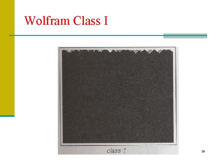
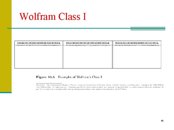
Wolfram’s CA Classification n Class I: Eventually every cell in the array settles into one state, never to change again. n n n Simple Uniform final state (all black or all white) Some examples are rules 0, 32, 128, 160, 254 Analogous to computer programs that halt after a few steps and to dynamical systems that have fixed-point attractors. after a finite number of time steps, the CA tends to achieve a unique state from nearly all possible starting conditions (limit points) 38

Wolfram Class I 39

Wolfram Class I 40

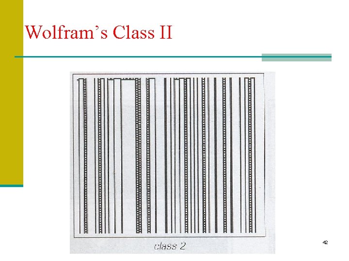
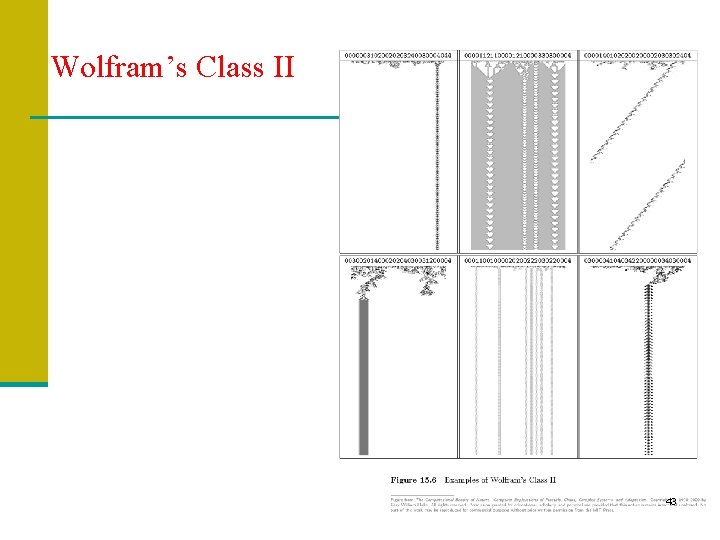
Wolfram’s CA Classification n Class II: Eventually the array settles into a periodic cycle of states (called a limit cycle). n n n Set of simple structures Structures remain the same or repeat every so often Examples include rules 132, 164, 218, 222 Analogous to computer programs that execute infinite loops and to dynamical systems that fall into limit cycles. the CA creates patterns that repeat periodically or are stable (limit cycles) – probably equivalent to a regular grammar/finite state automaton 41

Wolfram’s Class II 42

Wolfram’s Class II 43

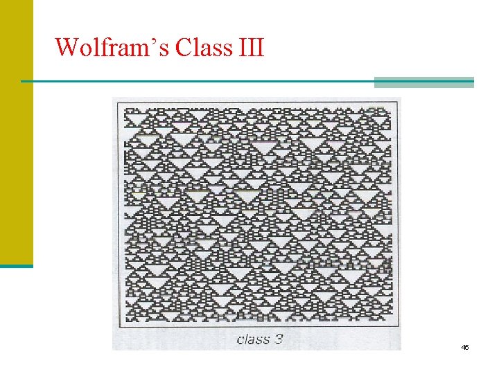
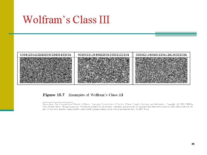
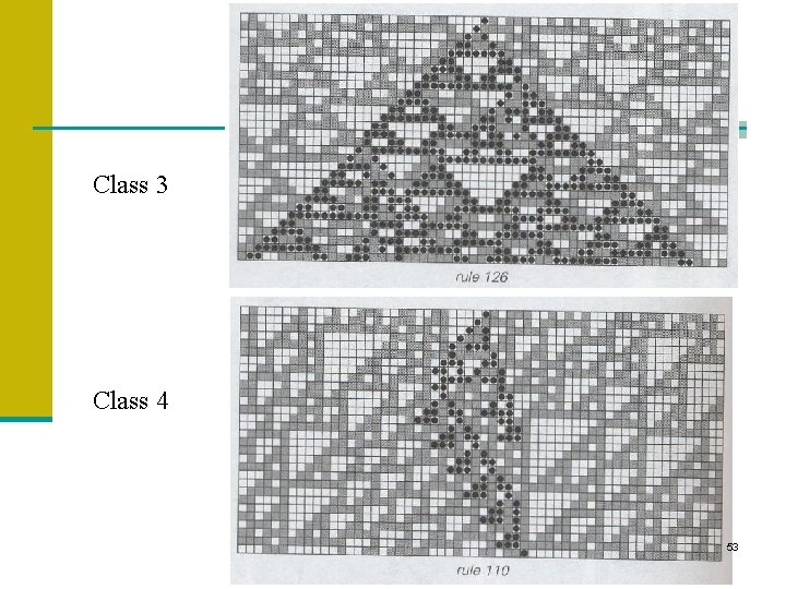
Wolfram’s CA Classification n Class III: The array forms “aperiodic” random-like patterns. n Appears random n Smaller structures can be seen some at some level n Most are expected to be computationally irreducible n Examples include rules 22, 30, 126 n Analogous to computer programs that are pseudo-random number generators (pass most tests for randomness, highly sensitive to seed, or initial condition). n Analogous to chaotic dynamical systems. Almost never repeat themselves, sensitive to initial conditions, embedded unstable limit cycles. n from nearly all starting conditions, the CA leads to aperiodic-chaotic patterns, where the statistical properties of these patterns are almost identical (after a sufficient period of time) to the starting patterns (self-similar fractal curves) – computes ‘irregular problems’ 44

Wolfram’s Class III 45

Wolfram’s Class III 46

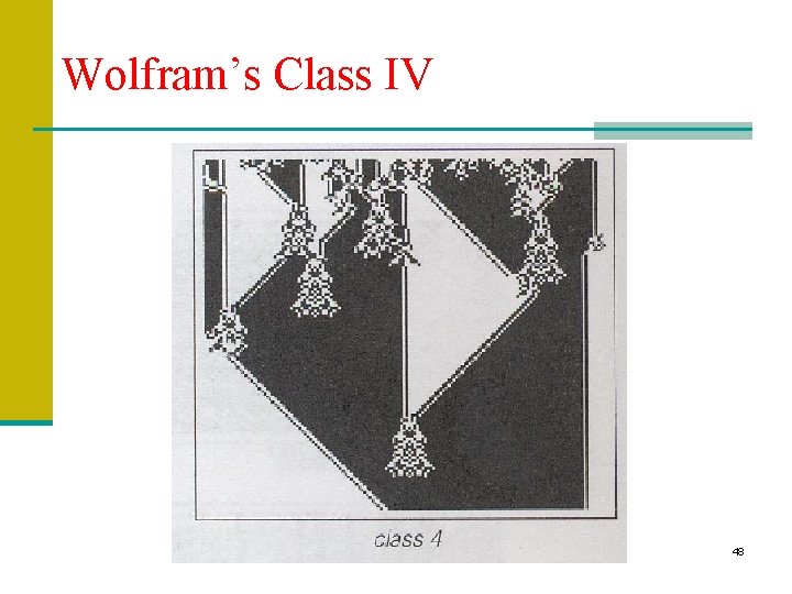
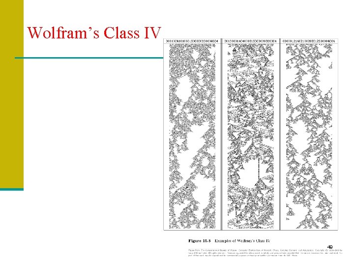
Wolfram’s Classification cont. n Class IV: The array forms complex patterns with localized structure that move through space and time: n Has order and randomness n Smaller scale structures interacting in complex ways Examples include codes 1815, 2007, 1659, 2043 Recall: Codes are “totalistic” CAs where new color depends on average of neighbors Class 4 emerges as an intermediate class between classes 2 and 3 Difficult to describe. Not regular, not periodic, not random. Speculate that it is interesting computation. after a finite number of steps, the CA usually dies, but there a few stable (periodic) patterns possible (e. g. Game of Life) - Class 4 CA are believed to be capable of universal computation n n n Hypothesis: The most interesting and complex behavior occurs in Class IV CA---the edge of chaos. n Example: Rule 110 47

Wolfram’s Class IV 48

Wolfram’s Class IV 49

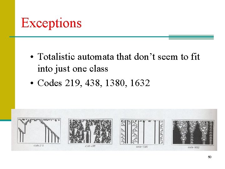
Exceptions • Totalistic automata that don’t seem to fit into just one class • Codes 219, 438, 1380, 1632 50

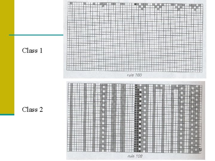
Initial condition sensitivity • Each class responds differently to a change in its initial conditions • Response types • Class 1 changes always die out • Changes continue on but are localized for Class 2 • Uniform rate of change affecting the whole system seen in Class 3 • Class 4 has nonuniform changes 51

Class 1 Class 2 52

Class 3 Class 4 53

Claim • Differences in responses of classes show each class handles information in a different way • Fundamental to our understanding of nature 54

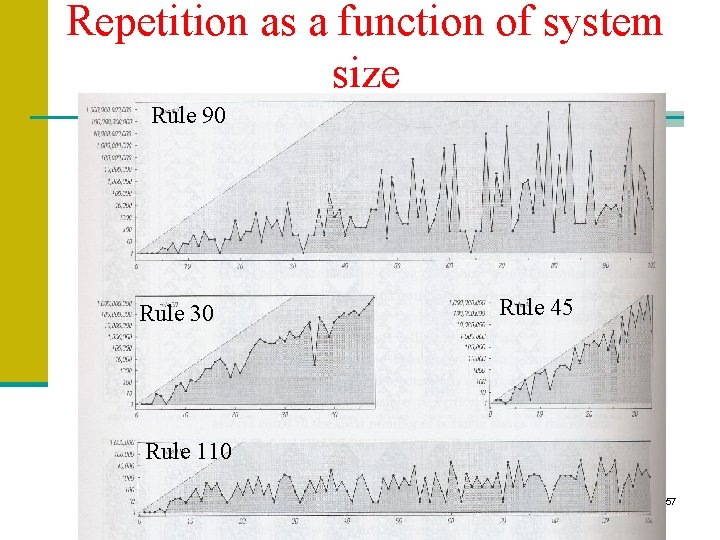
Class 2 • Repetitive behavior • No for support long-range communication • Lack of long-range communication makes systems of limited size forcing repetitiveness 55

Observing systems of limited behavior • Limiting the size forces repetivness • Period of repetition increases with size of system • With n cells, there at most 2 n possible states (maximum period of 2 n) • Modulus 56

Repetition as a function of system size Rule 90 Rule 30 Rule 45 Rule 110 57

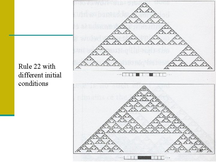
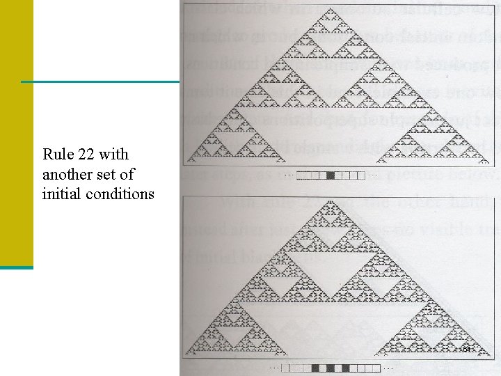
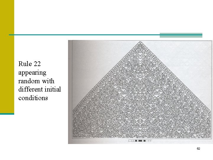
Class 3 randomness • Randomness exists even without random initial conditions • Different initial conditions can produce random behavior or nested pattern behavior in the same rule (rule 22) • Some rules need the random initial condition to exhibit randomness (90) and some rules don’t (30) 58

“Instrinsic Randomness” • Do systems like rule 22 or rule 30 have intrinsic randomness? • Do these examples prove that certain systems have intrinsic randomness and do not depend on initial conditions? • Special initial conditions can make class 3 systems behave like a class 2 or even a class 1 system (rule 126) 59

Rule 22 with different initial conditions 60

Rule 22 with another set of initial conditions 61

Rule 22 appearing random with different initial conditions 62

Class 4 structures • Certain structures will always last • Any way to predict the structures of a given rule and initial conditions? • One can find all structures given a period, but prediction is another matter 63

Attractors • Sequences of cells restricted as iterations progress, even with random initial conditions • Networks examples 64

Types of Networks • Classes 1 and 2 • Never have more than t 2 nodes after t steps • Classes 3 and 4 • Allowed sequences of cells becomes more complicated • Number of nodes increases at least exponentially 65

Class 3 and 4 Exceptions • Increase in network complexity not seen in special initial conditions for rules 204, 240, 30, and 90 • Onto mappings defined • Any other initial conditions than “special” initial conditions rapidly increase in complexity 66

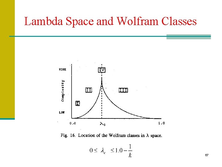
Lambda Space and Wolfram Classes 67

Lambda Parameter cont. n Table walkthrough illustrates interesting change in dynamics as function of lambda: n Transient lengths increase dramatically in middle of the range (see next slide). n However, different traversals of lambda space using the walkthrough method make the transition at different lambda values, although there is a well defined distribution around a mean value. n Size of the array has an effect on dynamics only for intermediate values of lambda. n Transient length depends exponentially on array size at lambda = 0. 5. n Overall evolutionary pattern in time is more random as lambda increases past the transition region (use entropy and mutual information). n Transition region supports both static and propagating structures. 68

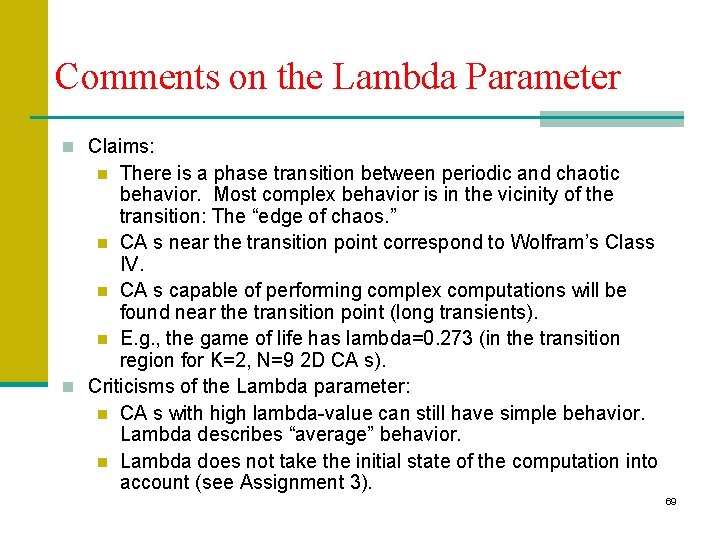
Comments on the Lambda Parameter n Claims: There is a phase transition between periodic and chaotic behavior. Most complex behavior is in the vicinity of the transition: The “edge of chaos. ” n CA s near the transition point correspond to Wolfram’s Class IV. n CA s capable of performing complex computations will be found near the transition point (long transients). n E. g. , the game of life has lambda=0. 273 (in the transition region for K=2, N=9 2 D CA s). n Criticisms of the Lambda parameter: n CA s with high lambda-value can still have simple behavior. Lambda describes “average” behavior. n Lambda does not take the initial state of the computation into account (see Assignment 3). n 69

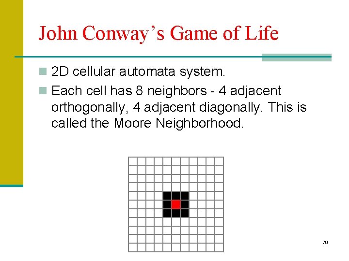
John Conway’s Game of Life n 2 D cellular automata system. n Each cell has 8 neighbors - 4 adjacent orthogonally, 4 adjacent diagonally. This is called the Moore Neighborhood. 70

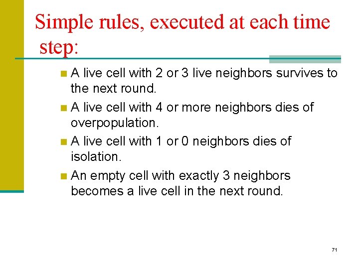
Simple rules, executed at each time step: A live cell with 2 or 3 live neighbors survives to the next round. n A live cell with 4 or more neighbors dies of overpopulation. n A live cell with 1 or 0 neighbors dies of isolation. n An empty cell with exactly 3 neighbors becomes a live cell in the next round. n 71

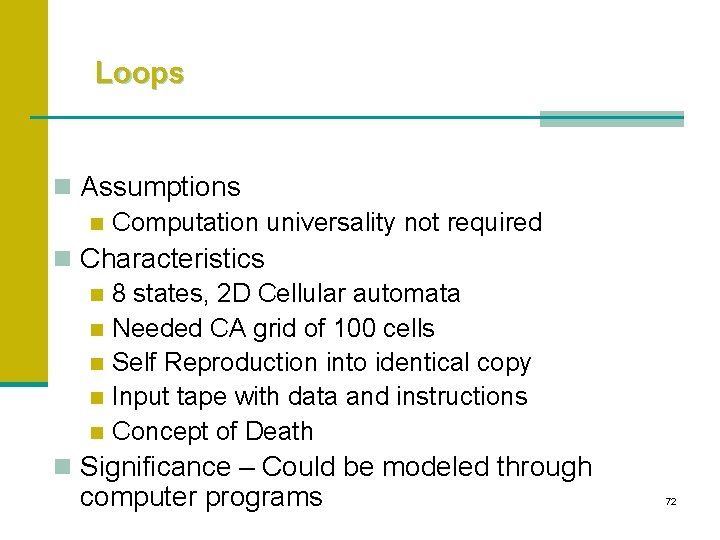
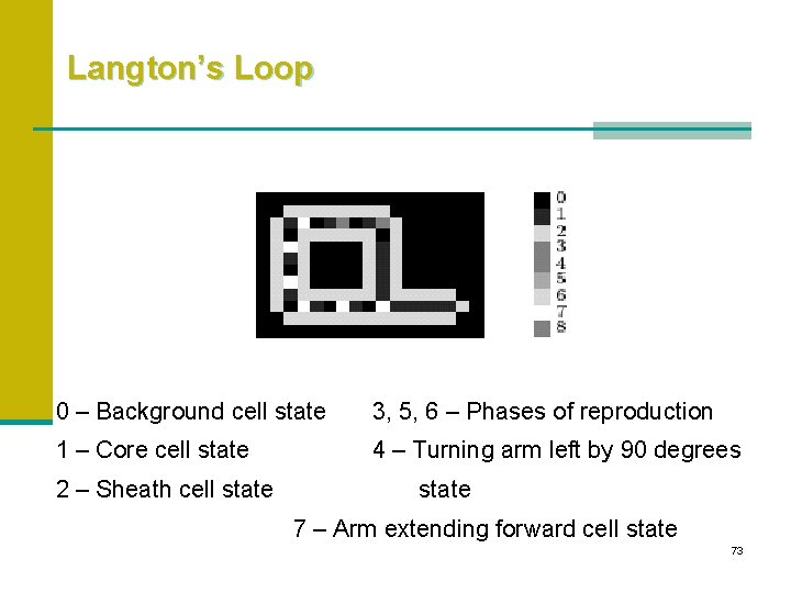
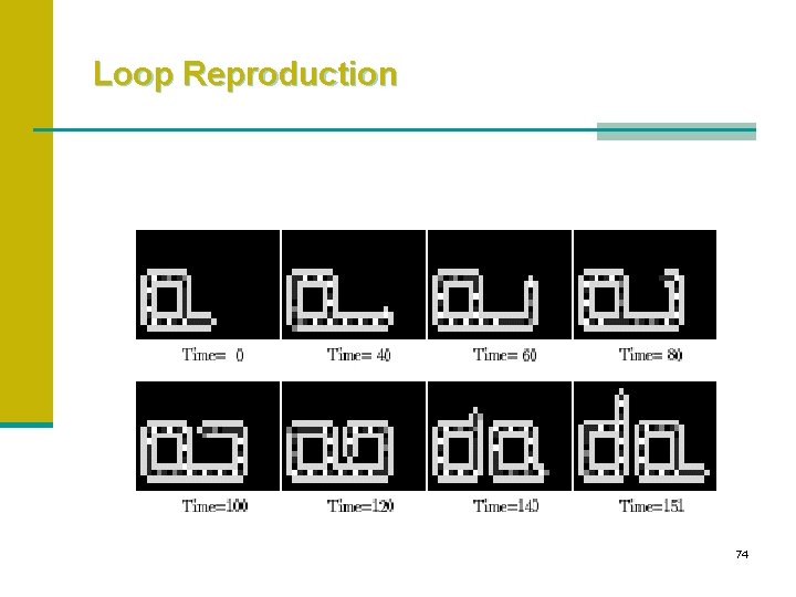
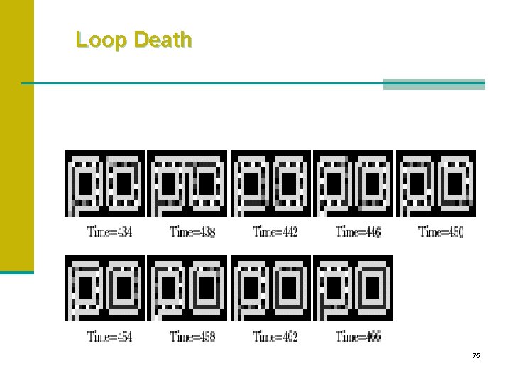
Loops n Assumptions n Computation universality not required n Characteristics n 8 states, 2 D Cellular automata n Needed CA grid of 100 cells n Self Reproduction into identical copy n Input tape with data and instructions n Concept of Death n Significance – Could be modeled through computer programs 72

Langton’s Loop 0 – Background cell state 3, 5, 6 – Phases of reproduction 1 – Core cell state 4 – Turning arm left by 90 degrees 2 – Sheath cell state 7 – Arm extending forward cell state 73

Loop Reproduction 74

Loop Death 75

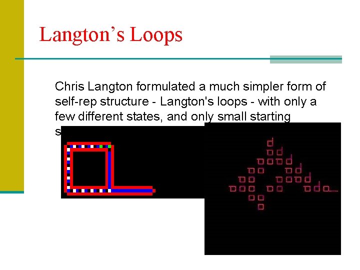
Langton’s Loops Chris Langton formulated a much simpler form of self-rep structure - Langton's loops - with only a few different states, and only small starting structures. 76

Example: Modelling Sharks and Fish: 77

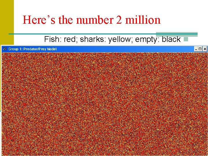
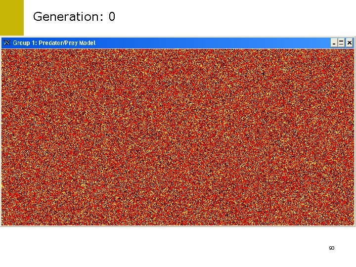
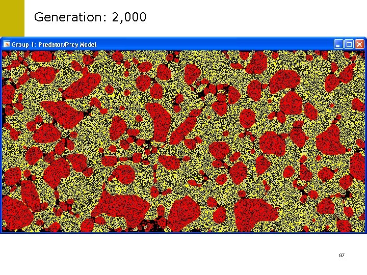
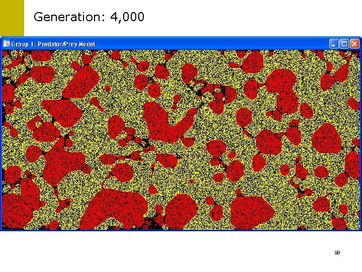
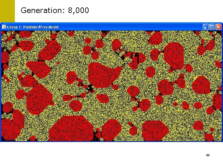
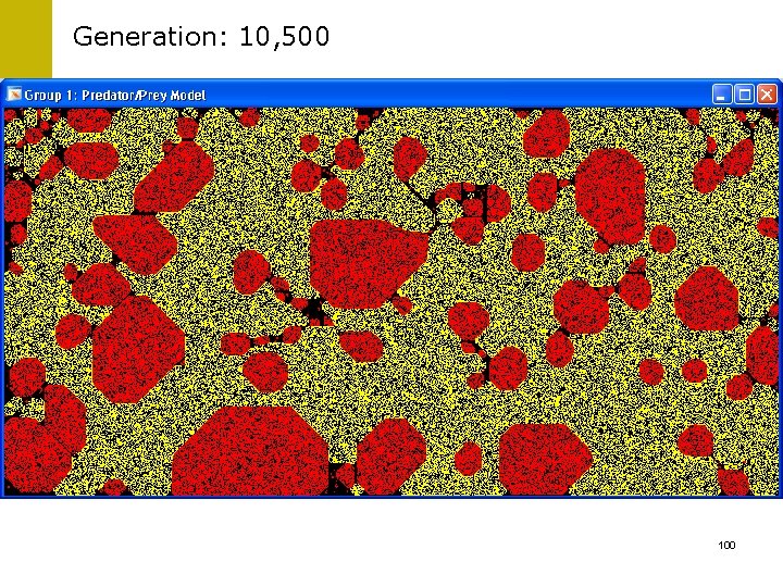
n modeled a predator/prey relationship n Begins with a randomly distributed population of fish, sharks, and empty cells in a 1000 x 2000 cell grid (2 million cells) n Initially, n n n 50% of the cells are occupied by fish 25% are occupied by sharks 25% are empty 78

Here’s the number 2 million Fish: red; sharks: yellow; empty: black n 79

Rules A dozen or so rules describe life in each cell: n birth, longevity and death of a fish or shark n breeding of fish and sharks n over- and under-population n fish/shark interaction n Important: what happens in each cell is determined only by rules that apply locally, yet which often yield long-term large-scale patterns. 80

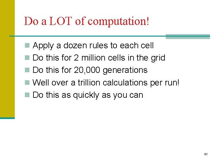
Do a LOT of computation! n Apply a dozen rules to each cell n Do this for 2 million cells in the grid n Do this for 20, 000 generations n Well over a trillion calculations per run! n Do this as quickly as you can 81

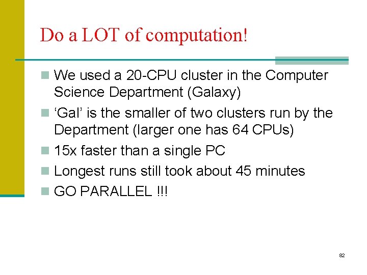
Do a LOT of computation! n We used a 20 -CPU cluster in the Computer Science Department (Galaxy) n ‘Gal’ is the smaller of two clusters run by the Department (larger one has 64 CPUs) n 15 x faster than a single PC n Longest runs still took about 45 minutes n GO PARALLEL !!! 82

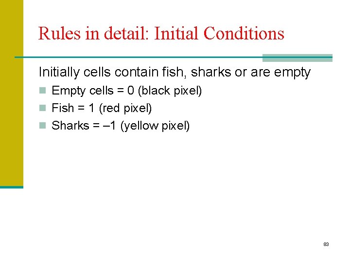
Rules in detail: Initial Conditions Initially cells contain fish, sharks or are empty n Empty cells = 0 (black pixel) n Fish = 1 (red pixel) n Sharks = – 1 (yellow pixel) 83

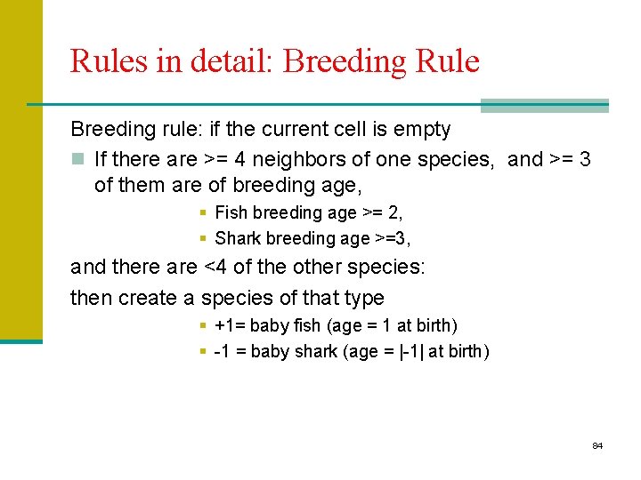
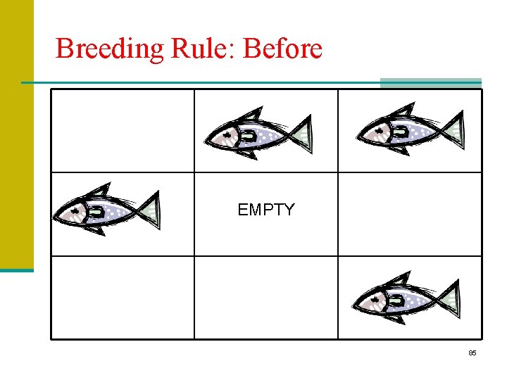
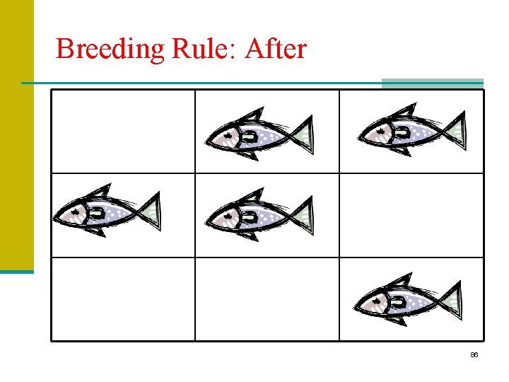
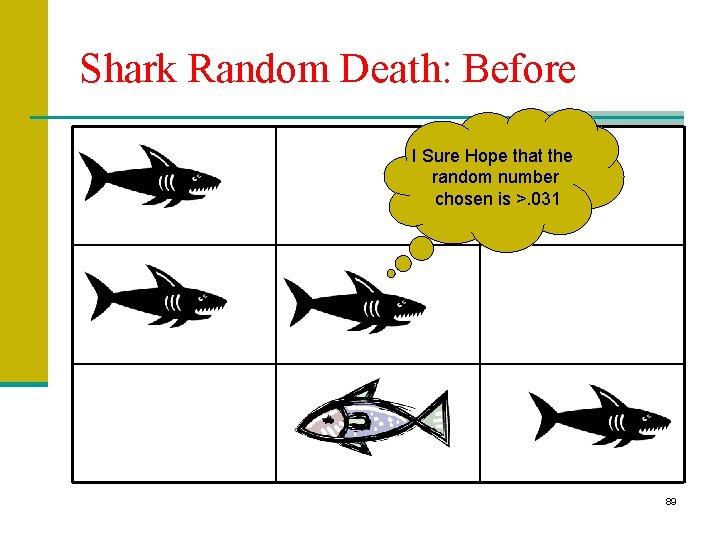
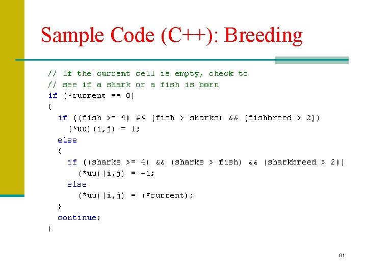
Rules in detail: Breeding Rule Breeding rule: if the current cell is empty n If there are >= 4 neighbors of one species, and >= 3 of them are of breeding age, § Fish breeding age >= 2, § Shark breeding age >=3, and there are <4 of the other species: then create a species of that type § +1= baby fish (age = 1 at birth) § -1 = baby shark (age = |-1| at birth) 84

Breeding Rule: Before EMPTY 85

Breeding Rule: After 86

Rules in Detail: Fish Rules If the current cell contains a fish: n Fish live for 10 generations n If >=5 neighbors are sharks, fish dies (shark food) n If all 8 neighbors are fish, fish dies (overpopulation) n If a fish does not die, increment age 87

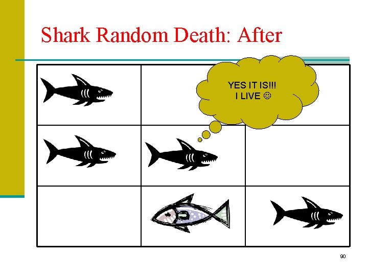
Rules in Detail: Shark Rules If the current cell contains a shark: n Sharks live for 20 generations n If >=6 neighbors are sharks and fish neighbors =0, the shark dies (starvation) n A shark has a 1/32 (. 031) chance of dying due to random causes n If a shark does not die, increment age 88

Shark Random Death: Before I Sure Hope that the random number chosen is >. 031 89

Shark Random Death: After YES IT IS!!! I LIVE 90

Sample Code (C++): Breeding 91

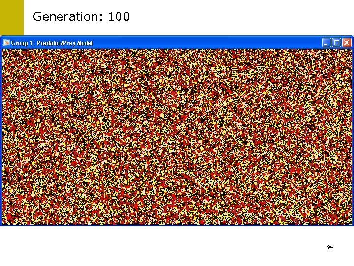
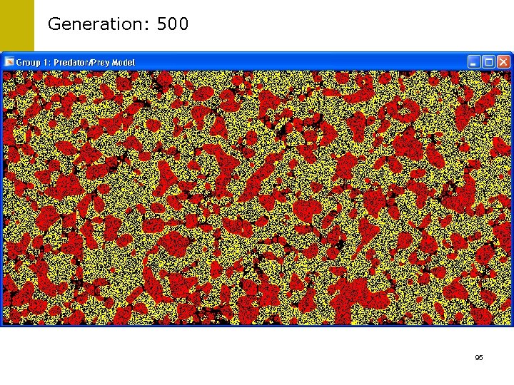
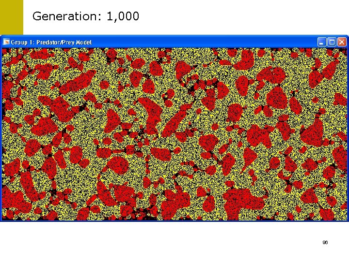
Results n Next several screens show behavior over a span of 10, 000+ generations 92

Generation: 0 93

Generation: 100 94

Generation: 500 95

Generation: 1, 000 96

Generation: 2, 000 97

Generation: 4, 000 98

Generation: 8, 000 99

Generation: 10, 500 100

Long-term trends n Borders tended to ‘harden’ along vertical, horizontal and diagonal lines n Borders of empty cells form between like species n Clumps of fish tend to coalesce and form convex shapes or ‘communities’ 101

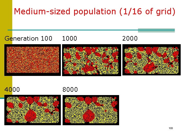
Variations of Initial Conditions n Still using randomly distributed populations: n Medium-sized population. Fish/sharks occupy: 1/16 th of total grid Fish: 62, 703; Sharks: 31, 301 n Very small population. Fish/sharks occupy: 1/800 th of total grid Initial population: Fish: 1, 298; Sharks: 609 102

Medium-sized population (1/16 of grid) Generation 1000 4000 8000 2000 103

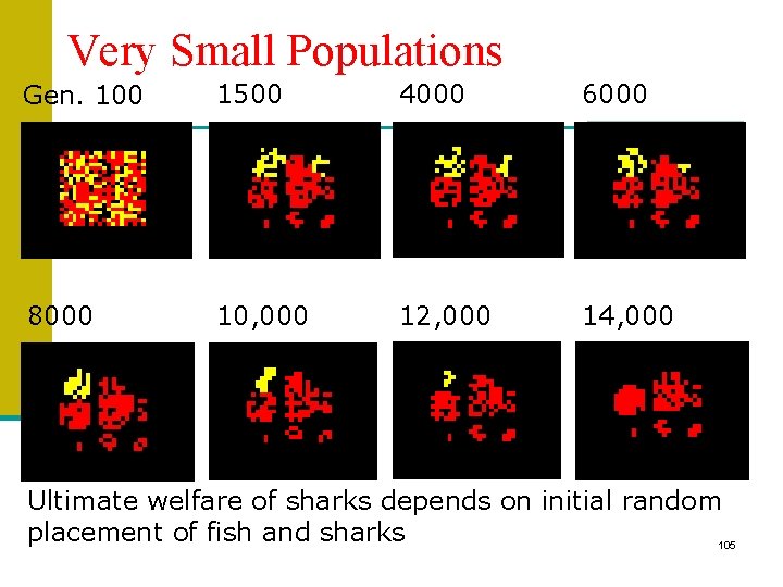
Very Small Populations n Random placement of very small populations can favor one species over another n Fish favored: sharks die out n Sharks favored: sharks predominate, but fish survive in stable small numbers 104

Very Small Populations Gen. 100 1500 4000 6000 8000 10, 000 12, 000 14, 000 Ultimate welfare of sharks depends on initial random placement of fish and sharks 105

Very small populations n Fish can live in stable isolated communities as small as 20 -30 n A community of less than 200 sharks tends not to be viable 106

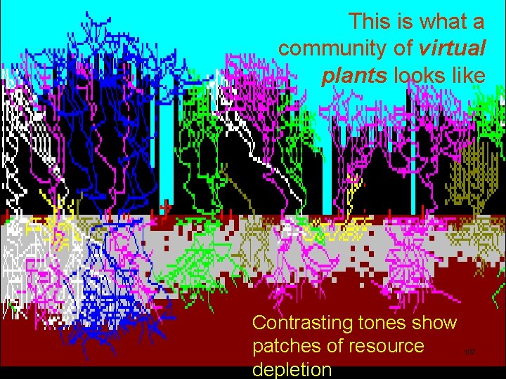
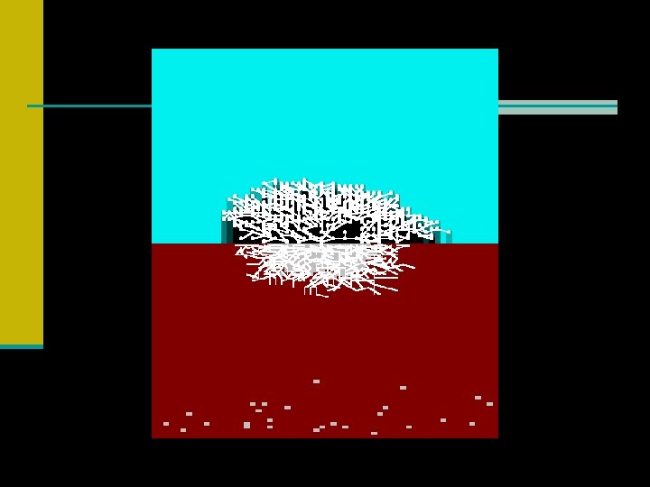
This is what a community of virtual plants looks like Community image Contrasting tones show patches of resource depletion 107

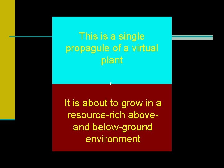
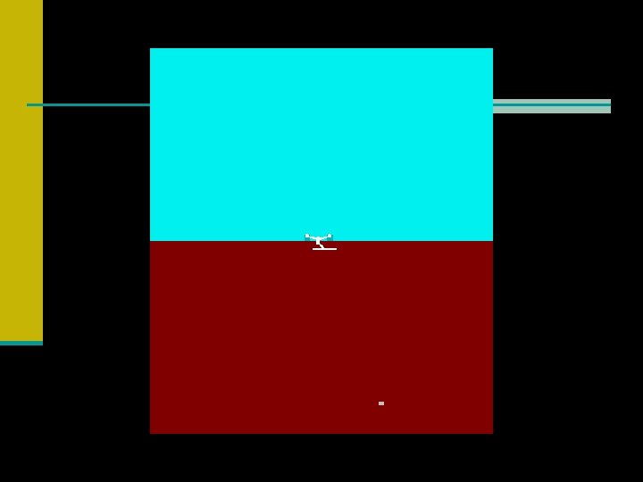
This is a single propagule of a virtual plant It is about to grow in a resource-rich aboveand below-ground environment 108

109

110

111

112

113

114

115

116

117

118

119

120

121

122

123

124

125

126

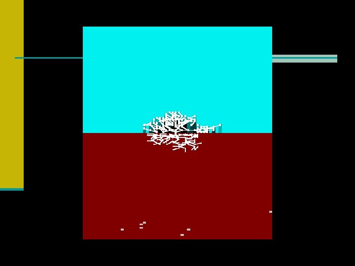
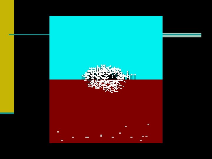
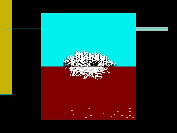
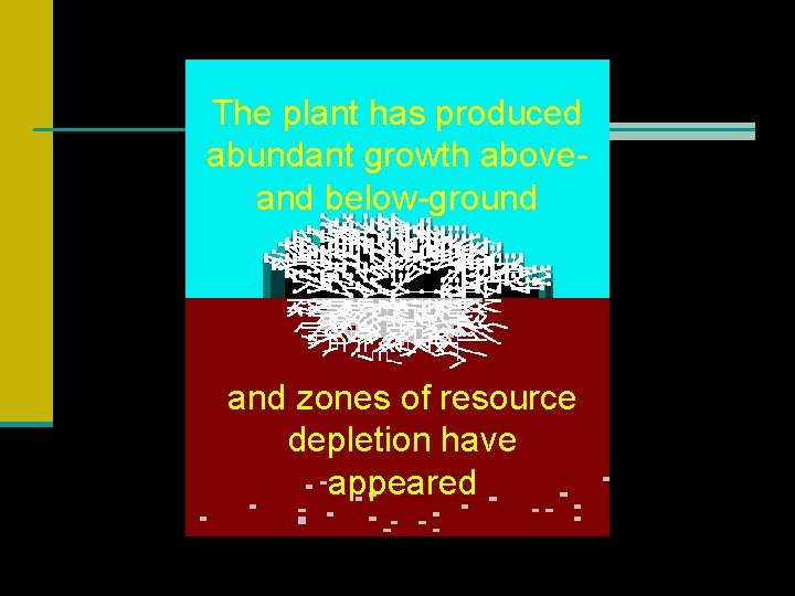
The plant has produced abundant growth aboveand below-ground and zones of resource depletion have appeared 127

See Rod Hunt at http: //www. ex. ac. uk/~rh 203/ for lots more about the plant life CA and its uses 128