The yeast Saccharomyces cerevisiae is commonly used as


 Major control point is at G 1/S morphology • reflects")


![% of Octads with MII pattern/2 = [c. M]](https://slidetodoc.com/presentation_image_h/7a5b4b97f233cfbd00846672778c32aa/image-28.jpg "% of Octads with MII pattern/2 = [c. M]")


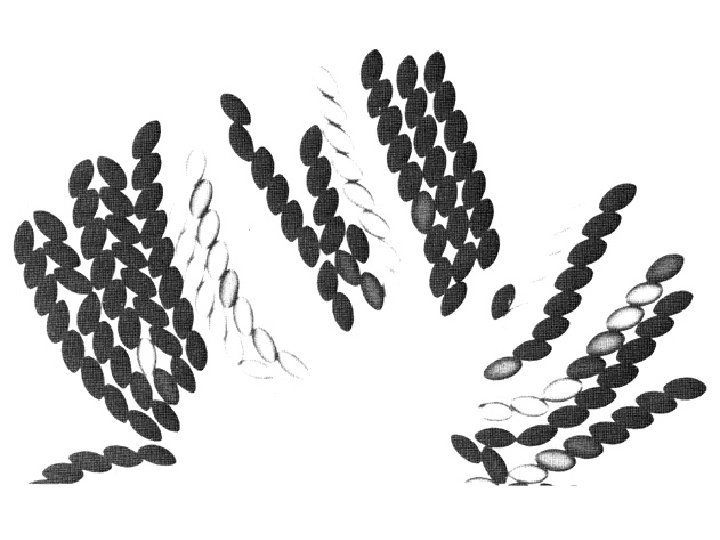
 -here UNORDERED tetrads Step 1: separate spores by micromanipulation")


 Tetrad Dissection BA BA ba ba Ba Ba b. A")
, but. . MESSAGE Linear and unordered tetrads can")


 Tetrad Dissection BA BA ba ba Ba Ba b. A")
 Phenotype – multiple gene")


- Slides: 69
The yeast Saccharomyces cerevisiae is commonly used as a model system =Budding Yeast =Bakers Yeast
Major advantages of the budding yeast as a genetic system • Grows fast • Cheap • Compact genome, fully sequenced since 1996. • Easy to handle • Superb Genetics, Biochemistry, Molecular Biology • Easy to transform, high efficiency of gene targeting
Major characteristic of the budding yeast • Unicellular Eukaryote • Grows by budding • 16 linear chromosomes • Generation Time: ~100 min • Can exist as stable diploid or haploid
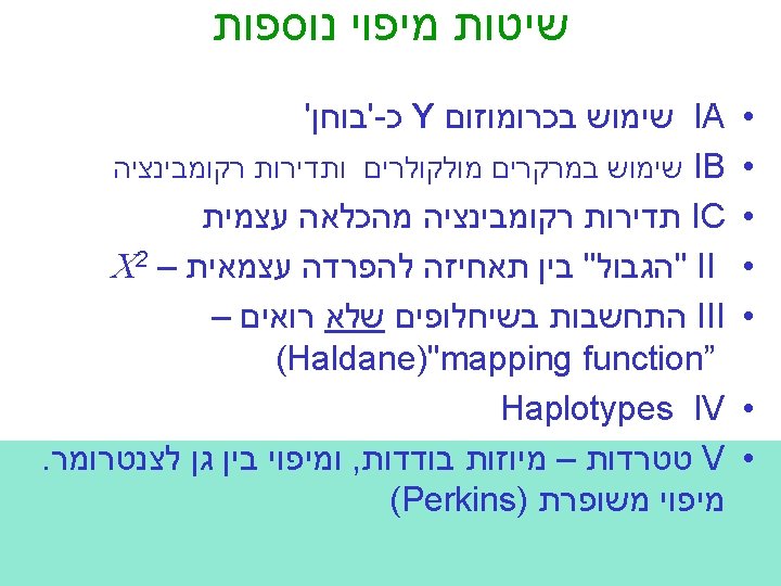
What is yeast? • • • Yeast - a fungus that divides to yield individual separated cells (as opposed to molds- mycelium) Saccharomyces cerevisiae (budding yeast) baker’s yeast closely related to brewer’s yeasts grows on rotting fruits Schizosaccharomyces pombe (fission yeast) African brewer’s yeast Saccharomyces relatives (S. bayanus, S. paradoxus, etc. ) Candida albicans Cryptococcus neoformans
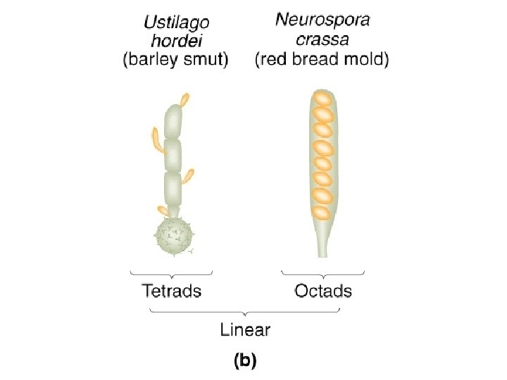
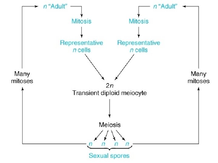
Yeast life cycle
• Mendel’s rules are relevant for organisms that sexually reproduce: diploid/haploid Plants, Animals, many Mora… – Those that ‘do’ meiosis
Haploid Mitosis
Diploid Mitosis
Haploid Mitosis Diploid Mitosis
Of diploid Of haploid 1 n 1 n 1 n 2 1
Animation 3. 3
Yeast cell cycle (mitosis) Major control point is at G 1/S morphology • reflects cell cycle position same in haploids • and diploids major control • point is ‘start’-cells can choose – mitosis, meiosis or mating depends on ploidy, env. & presence of partner – Morphology + nuclear localization and MT localization indicates the precise stage of the cell cycle
Centromere mapping
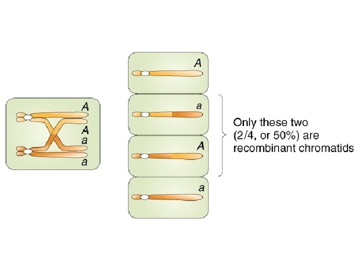
Centromere mapping Nonsister chromatids do not cross over First-division segregation pattern or MI pattern
Centromere mapping n = 2 -> 4 S 2 1 1 1
Centromere mapping Nonsister chromatids do not cross over First-division segregation pattern or MI pattern
HALF OF Animation 3. 3 – to 37”
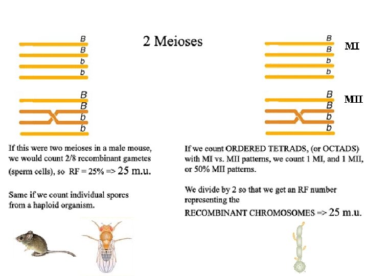
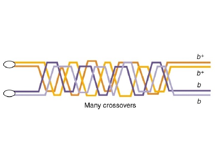
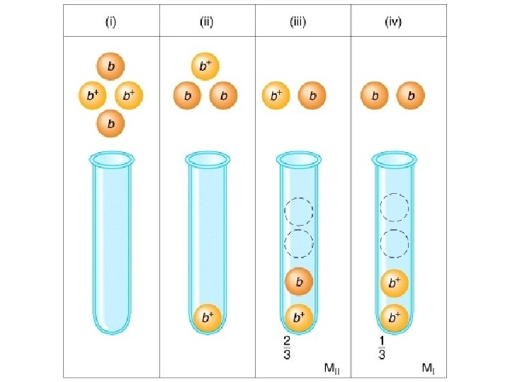
Centromere mapping Nonsister chromatids cross over Second-division segregation pattern or MII pattern
Second-division segregation pattern or MII pattern
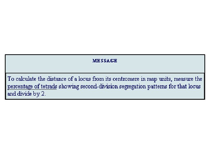
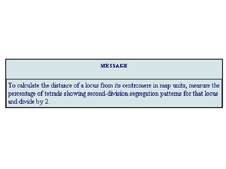
% of Octads with MII pattern/2 = [c. M]
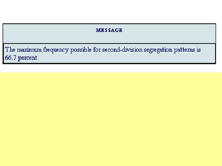
The numerical limits of this method. . . ?
We’ve learned much more from tetrads/octads. -Let’s go to 2 genes. . . 1. The loci are on separate chromosomes 2. The loci are on opposite sides of the centromere on the same chromosome 3. The loci are on the same side of the centromere on the same chromosome
Yeast tetrad analysis (classic method) -here UNORDERED tetrads Step 1: separate spores by micromanipulation with tetrad a glass needle Step 2: place the four spores from each tetrad in a row on an agar plate Step 3: let the spores grow into colonies
or PDT
Unordered tetrads B a Mating b A B a b A Heterozygous diploid Meiosis B B b b a a A A Tetrad Dissection BA BA ba ba NPD Ba Ba b. A PDT BA Ba ba b. A TT
Classical approach (tetrad dissection) Tetrad Dissection BA BA ba ba Ba Ba b. A BA Ba ba b. A NPD PDT TT Tetrad bni 1∆ bnr 1∆ Only double mutant ( b a ) does not survive
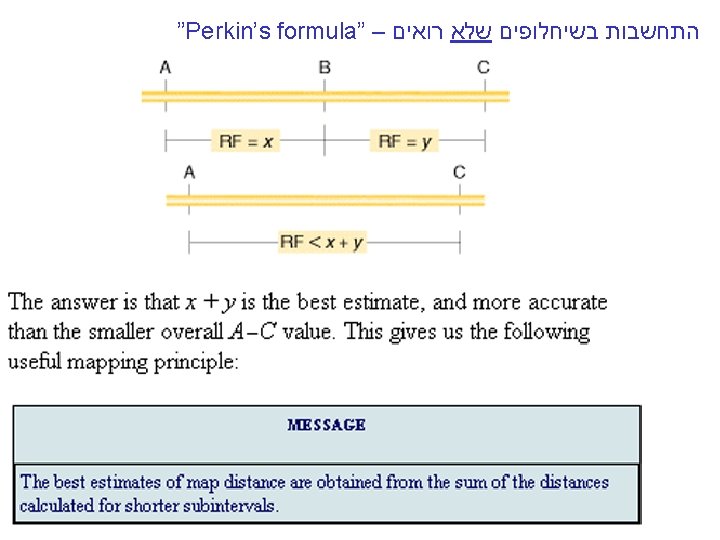
Simple RF= 100(NPD + ½ T), but. . MESSAGE Linear and unordered tetrads can be used to calculate the frequencies of single and double crossovers, which can be used to calculate accurate map distances. Perkin formula Corrected map distance=50(T+6 NPD) m. u. [c. M]
Derivation of Perkin’s formula Now, what do these types tell us about linkage? You will notice from examining the three types that only the NPD and T types contain recombinants, so they are key classes in determining recombinant frequency. The NPD class contains only recombinants, whereas half the spores in the T class are recombinant. Therefore, we can write a formula for determining RF by using tetrads, where T and NPD represent the percentages of those classes: Image ch 6 e 14. jpg If this formula gives a frequency of 50 percent, then we know that the loci must be unlinked, and correspondingly, if the RF is less than 50 percent, then the genes must be linked and we could use that value to represent the number of map units between them. However, just as with other linkage analyses studied earlier in the chapter, this value is an underestimate, because it does not consider double recombinants and other higher-level crossovers. Nevertheless, the frequencies of PD, NPD, and T can be used to make a correction for doubles. First, we need to understand how the PD, NPD, and T classes are produced in crosses in which there are linked markers. Let us assume that genes a and b are linked. If we assume that individual meioses can have no crossovers (NCO), a single crossover (SCO), or a double crossover (DCO) in the a-to-b region, then we can represent the classes of unordered asci that emerge from such meioses as shown in Figure 6 -14. Triples and higher numbers of crossovers might occur, but we may assume that such crossovers are rare and therefore negligible. SEE Figure 6 -14 in the bottom corner. The ascus classes produced by crossovers between linked loci. NCO, noncrossover meioses; SCO, single-crossover meioses; DCO, double-crossover meioses. The key to the analysis is the NPD class, which arises only from a double crossover between all four chromatids. Because we are assuming that double crossovers occur randomly between the chromatids, we can also assume that the frequencies of the four DCO classes are equal. This assumption means that the NPD class should contain 1/4 of the DCOs, and therefore we can estimate that The single-crossover class also can be calculated by a similar kind of reasoning. Notice that tetratype (T) asci can result from either single-crossover or double-crossover meioses. But we can estimate the component of the T class that comes from DCO meioses to be 2 NPD. Hence, the size of the SCO class can be stated as Now that we have estimated the sizes of the SCO and DCO classes, the noncrossover class can be estimated as Thus, we have estimates of the sizes of the NCO, SCO, and DCO classes in this marked region. We can use these values to derive a value for m, the mean number of crossovers per meiosis in this region. We can calculate the value of m simply by taking the sum of the SCO class plus twice the DCO class (because this class contains two crossovers). Hence: In the mapping-function section, we learned that, to convert an m value into map units, m must be multiplied by 50 because each crossover on average produces 50 percent recombinants. So:
Derivation of Perkin’s formula – using it, and comparing to RF Let’s assume that, in our hypothetical cross of a+ b+ × a b, the observed frequencies of the ascus classes are 56 percent PD, 41 percent T, and 3 percent NPD. Using the formula, we find the map distance between the a and b loci to be: Let us compare this value with that obtained directly from the RF. Recall that the formula is: In our example, This RF value is 6 m. u. , less than the estimate we obtained by using the mapdistance formula because we could not correct for double crossovers in the RF analysis.
What PD, NPD and T values are expected when dealing with unlinked genes? B B b b Mating aa aa Meiosis a. A B B aa aa b b A a. A Tetrad Heterozygous diploid Tetrad Dissection BA BA ba ba NPD Ba Ba b. A PDT BA Ba ba b. A TT
What PD, NPD and T values are expected when dealing with unlinked genes? What PD, NPD, and T values are expected when we deal with unlinked genes? The sizes of the PD and NPD classes will be equal as a result of independent assortment. The T class can be produced only from a crossover between either of the two loci and their respective centromeres, and therefore the size of the T class will depend on the total size of these two regions. B B aa aa Meiosis b Mating The sizes of the PD and NPD classes b will be equal as a result a. A of independent assortment. a. A The T class can be produced only form a crossover between the specific loci and their respective centromeres B B b b aa aa a A A Tetrad Heterozygous diploid Tetrad Dissection BA BA ba ba NPD Ba Ba b. A PDT BA Ba ba b. A TT
Classical approach (tetrad dissection) Tetrad Dissection BA BA ba ba Ba Ba b. A BA Ba ba b. A NPD PDT TT Tetrad bni 1∆ bnr 1∆ Only double mutant ( b a ) does not survive, Synthetic Lethality
Synthetic Lethality yfg 2 yfg 1 Viable Dead Synthetic (sick) Phenotype – multiple gene causality
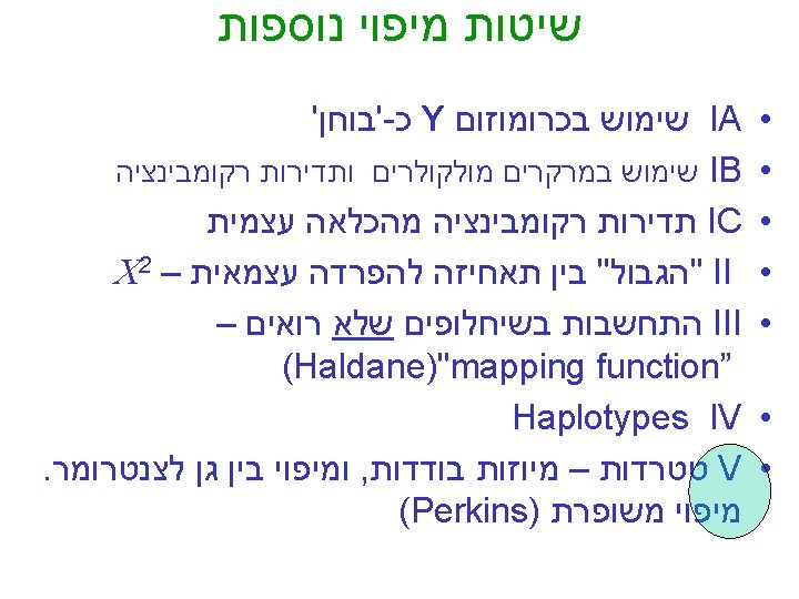
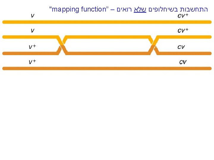
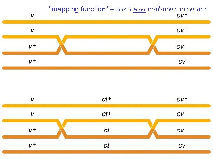
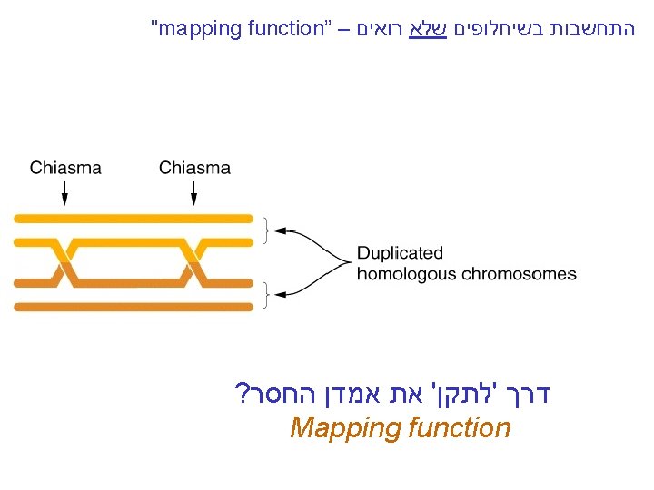
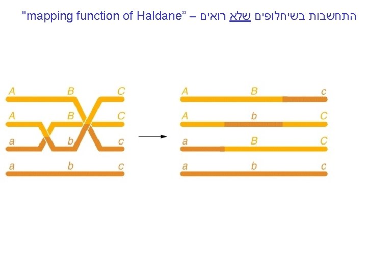
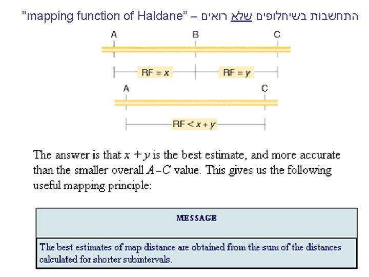
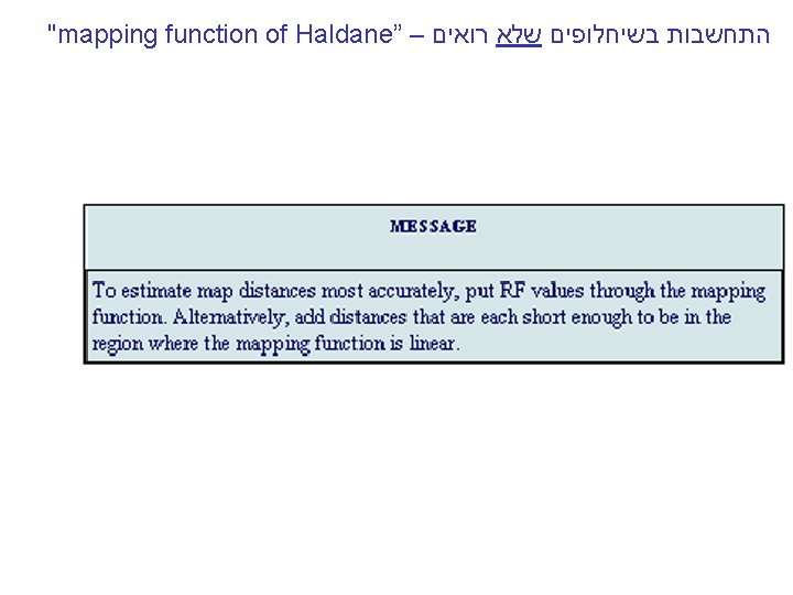
"mapping function of Haldane” – התחשבות בשיחלופים שלא רואים • POINT 1: Between two genes together in meioses: *If no crossovers occur between them, no recombinants result. *If one or more crossovers occur, 50% of the offspring will be recombinant (not intuitive). • POINT 2: From RF, we can derive the class of zero crossoversus 1 -or-more crossovers, using. . . • POISSON - predict the Gaussian curve of classes of crossovers, especially CLASS of ZERO crossovers, and calculate a corrected map distance – *The average number of crossovers between 2 genes.
POINT 1
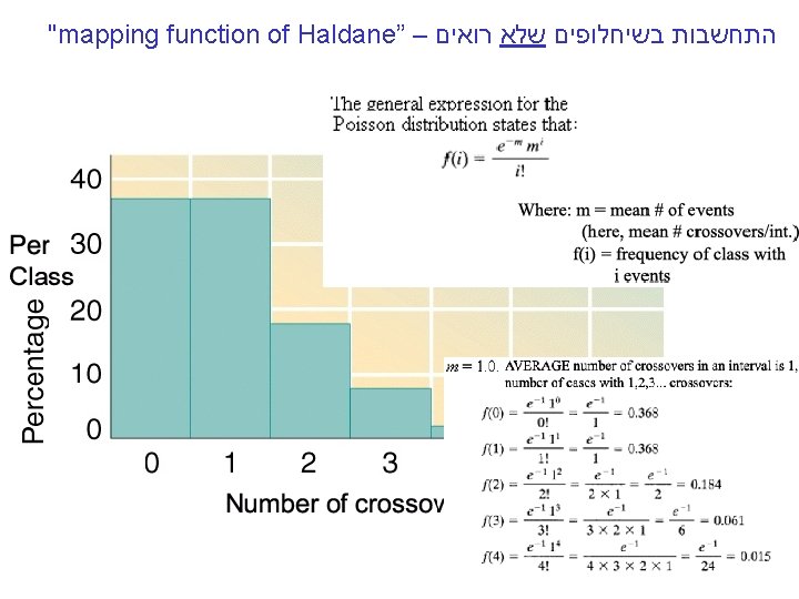
"mapping function of Haldane” – התחשבות בשיחלופים שלא רואים POINT 12 • POINT Between two of genes The 1: true determinant RF isin themeioses: relative *If nosizes crossovers occur, nono recombinants of the classes with crossovers, result. with any nonzero *If one orversus moreclasses crossovers occur, 50% of the of cross overs offspring will. Number be recombinant (not intuitive). • POINT 2: From RF, we can derive the class of zero crossoversus 1 -or-more crossovers, using. . . RF = 1/2 (Cases of 1 or more crossovers) RF = 1/2(1 – class with zero crossovers) When crossovers are relatively rare, the POISSON DISTRIBUTION formula Predicts the occurrence of each class: We’re interested -m i fi = (e m )/i! in the ‘Zero’ class
"mapping function of Haldane” – התחשבות בשיחלופים שלא רואים POINT 2
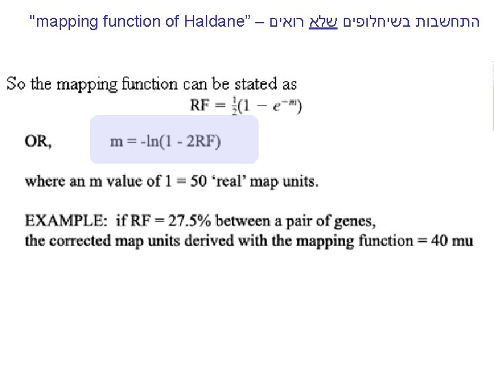
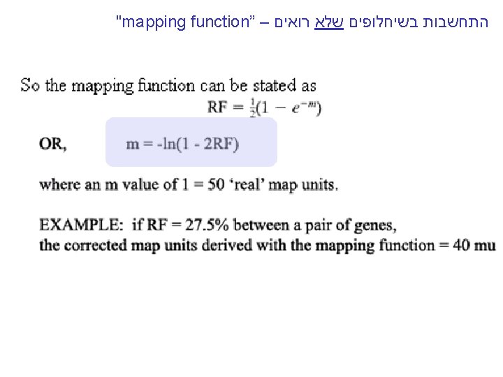
"mapping function of Haldane” – התחשבות בשיחלופים שלא רואים For Zero class: RF = 1/2(1 – class with zero crossovers)
"mapping function of Haldane” – התחשבות בשיחלופים שלא רואים • POINT 1: Between two genes in meioses: *If no crossovers occur, no recombinants result. *If one or more crossovers occur, 50% of the offspring will be recombinant (not intuitive). • POINT 2: From RF, we can derive the class of zero crossoversus 1 -or-more crossovers, using. . . • POISSON - predict the Gaussian curve of classes of crossovers, especially CLASS of ZERO crossovers, and calculate a corrected map distance – *The average number of crossovers between 2 genes.
"mapping function of Haldane” – התחשבות בשיחלופים שלא רואים The larger m get e-m tends to 0 and RF tends to 1/2 , or 50 m. u m-is the mean number of cross overs that occur in a segment per meiosis
OVERALL MESSAGE The inherent tendency of multiple crossovers to lead to an underestimate of map distance can be circumvented by the use of: Map function of Haldane (in any organism), and by the Perkin formula (in tetrad-producing organisms such as fungi)