Statistical Analysis of Microarray Data KaLok Ng Asia

Statistical Analysis of Microarray Data Ka-Lok Ng Asia University

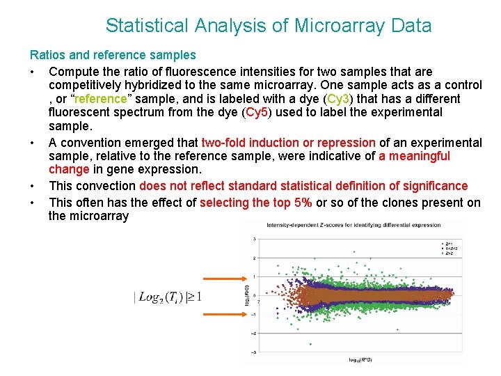
Statistical Analysis of Microarray Data Ratios and reference samples • Compute the ratio of fluorescence intensities for two samples that are competitively hybridized to the same microarray. One sample acts as a control , or “reference” sample, and is labeled with a dye (Cy 3) that has a different fluorescent spectrum from the dye (Cy 5) used to label the experimental sample. • A convention emerged that two-fold induction or repression of an experimental sample, relative to the reference sample, were indicative of a meaningful change in gene expression. • This convection does not reflect standard statistical definition of significance • This often has the effect of selecting the top 5% or so of the clones present on the microarray

Statistical Analysis Microarray Data Reasons for adopting ratios as the standard for comparison of gene expression (1) Microarrays do not provide data on absolute expression levels. Formulation of a ratio captures the central idea that it is a change in relative level of expression that is biological interesting. (2) removes variation among arrays from the analysis. Differences between microarray – such as (1) the absolute amount of DNA spotted on the arrays, (2) local variation introduced either during the sliding preparation and washing, or during image capture.

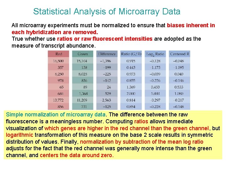
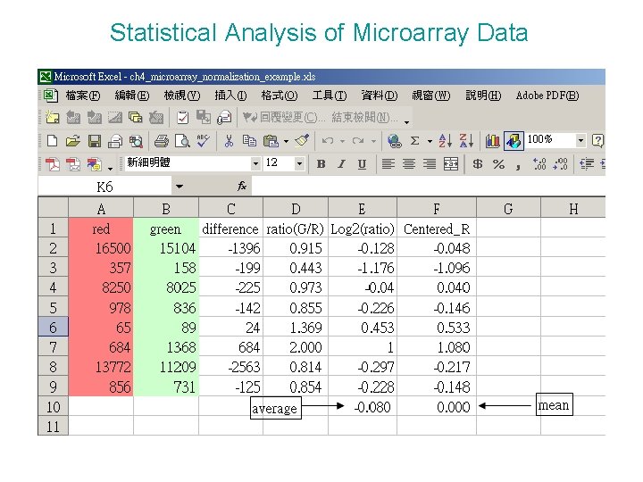
Statistical Analysis of Microarray Data All microarray experiments must be normalized to ensure that biases inherent in each hybridization are removed. True whether use ratios or raw fluorescent intensities are adopted as the measure of transcript abundance. Simple normalization of microarray data. The difference between the raw fluorescence is a meaningless number. Computing ratios allows immediate visualization of which genes are higher in the red channel than the green channel, but logarithmic transformation of this measure on the base 2 scale results in symmetric distribution of values. Finally, normalization by subtraction of the mean log ratio adjusts for the fact that the red channel was generally more intense than the green channel, and centers the data around zero.

Statistical Analysis of Microarray Data

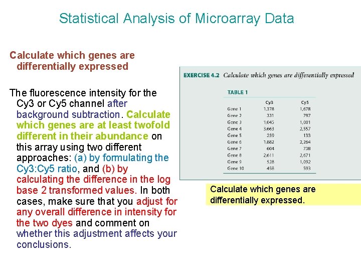
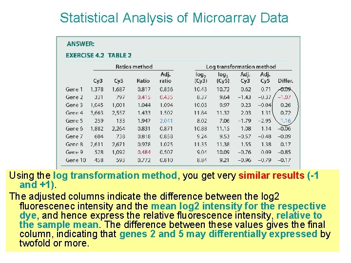
Statistical Analysis of Microarray Data Calculate which genes are differentially expressed The fluorescence intensity for the Cy 3 or Cy 5 channel after background subtraction. Calculate which genes are at least twofold different in their abundance on this array using two different approaches: (a) by formulating the Cy 3: Cy 5 ratio, and (b) by calculating the difference in the log base 2 transformed values. In both cases, make sure that you adjust for any overall difference in intensity for the two dyes and comment on whether this adjustment affects your conclusions. Calculate which genes are differentially expressed.

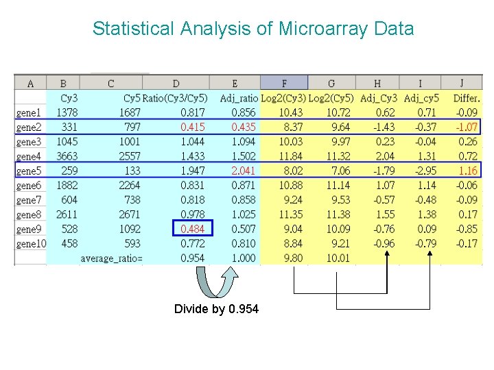
Statistical Analysis of Microarray Data Divide by 0. 954

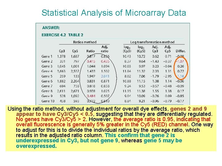
Statistical Analysis of Microarray Data Using the ratio method, without adjustment for overall dye effects, genes 2 and 9 appear to have Cy 3/Cy 5 < 0. 5, suggesting that they are differentially regulated. No genes have Cy 3/Cy 5 > 2. However, the average ratio is 0. 95, indicating that overall fluorescence is generally 5% greater in the Cy 5 (RED) channel. One way to adjust for this is to divide the individual ratios by the average ratio, which results in the adjusted ratio column. This confirm that gene 2 is underexpressed in Cy 3, but not gene 9, whereas gene 5 may be overexpressed.

Statistical Analysis of Microarray Data Using the log transformation method, you get very similar results (-1 and +1). The adjusted columns indicate the difference between the log 2 fluorescenec intensity and the mean log 2 intensity for the respective dye, and hence express the relative fluorescence intensity, relative to the sample mean. The difference between these values gives the final column, indicating that genes 2 and 5 may differentially expressed by twofold or more.

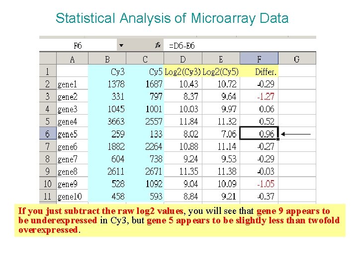
Statistical Analysis of Microarray Data If you just subtract the raw log 2 values, you will see that gene 9 appears to be underexpressed in Cy 3, but gene 5 appears to be slightly less than twofold overexpressed.

Finding significant genes • After normalizing, filtering and averaging the data, one can identify genes with expression ratios that are significantly different from 1 or -1 • Some genes fluctuates a great deal more than others (Hughes et al. 2000 a, b) • In general the genes whose expression is most variable are those in which expression is stress induced, modulated by the immune system or hormonally regulated (Pritchard et al. 2001) • There is the Missing Value problem in microarray data set – By interpolation References • Hughes TR, et al. (2000 a) Functional discovery via a compendium of expression profiles. Cell 102(1): 109 -26 • Hughes TR, et al. (2000 b) Widespread aneuploidy revealed by DNA microarray expression profiling. Nat Genet 25(3): 333 -7 • Pritchard et al. 2001 Project normal: Defining normal variance in mouse gene expression. PNAS 98, 13266.

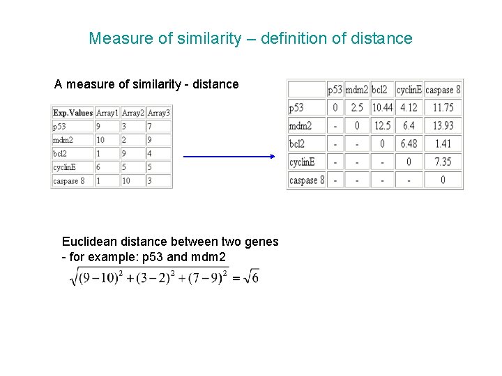
Measure of similarity – definition of distance A measure of similarity - distance Euclidean distance between two genes - for example: p 53 and mdm 2

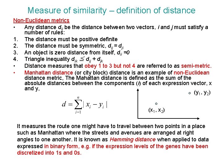
Measure of similarity – definition of distance Non-Euclidean metrics • Any distance dij be the distance between two vectors, i and j must satisfy a number of rules: 1. The distance must be positive definite 2. The distance must be symmetric, dij = dji 3. An object is zero distance from itself, dii =0 4. Triangle inequality dik ≦ dij + djk • Distance measures that obey 1 to 3 but not 4 are referred to as semi-metric. • Manhattan distance (or city block) distance is an example of non-Euclidean distance metric, The Mahattan distance is defined as the sum of the absolute distances between the components (i) of each expression vector, x and y, (y 1, y 2) (x 1, x 2) It measures the route one might have to travel between two points in a place such as Manhattan where the streets and avenues are arranged at right angles to one another. It is known as Hamming distance when applied to data expressed in binary form, e. g. if the expression levels of the genes have been discretized into 1 s and 0 s.

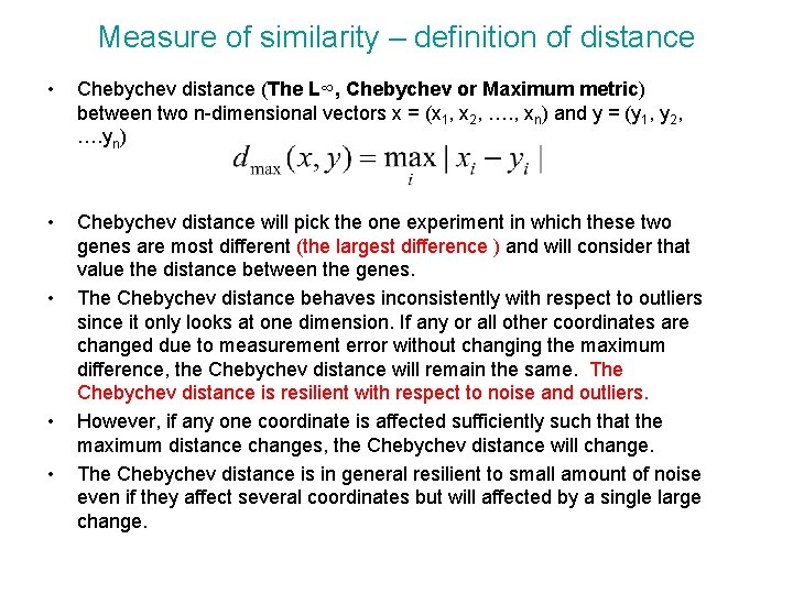
Measure of similarity – definition of distance • Chebychev distance (The L∞, Chebychev or Maximum metric) between two n-dimensional vectors x = (x 1, x 2, …. , xn) and y = (y 1, y 2, …. yn) • Chebychev distance will pick the one experiment in which these two genes are most different (the largest difference ) and will consider that value the distance between the genes. The Chebychev distance behaves inconsistently with respect to outliers since it only looks at one dimension. If any or all other coordinates are changed due to measurement error without changing the maximum difference, the Chebychev distance will remain the same. The Chebychev distance is resilient with respect to noise and outliers. However, if any one coordinate is affected sufficiently such that the maximum distance changes, the Chebychev distance will change. The Chebychev distance is in general resilient to small amount of noise even if they affect several coordinates but will affected by a single large change. • • •

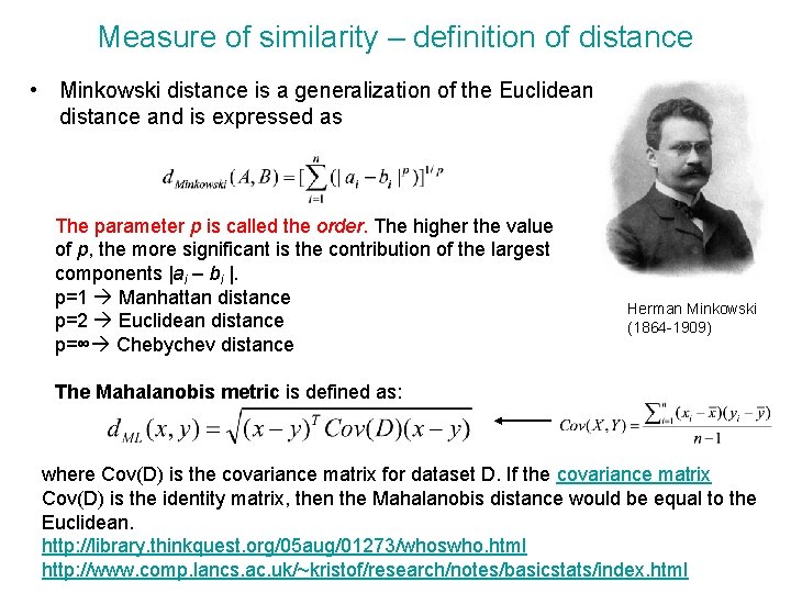
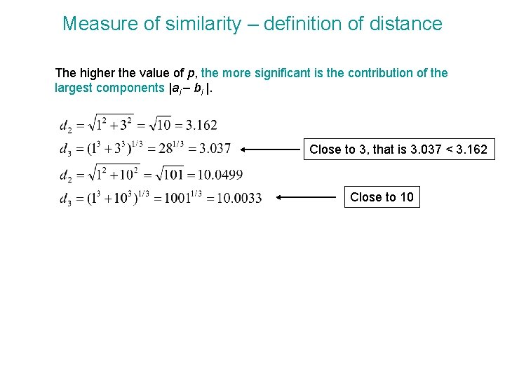
Measure of similarity – definition of distance • Minkowski distance is a generalization of the Euclidean distance and is expressed as The parameter p is called the order. The higher the value of p, the more significant is the contribution of the largest components |ai – bi |. p=1 Manhattan distance p=2 Euclidean distance p=∞ Chebychev distance Herman Minkowski (1864 -1909) The Mahalanobis metric is defined as: where Cov(D) is the covariance matrix for dataset D. If the covariance matrix Cov(D) is the identity matrix, then the Mahalanobis distance would be equal to the Euclidean. http: //library. thinkquest. org/05 aug/01273/whoswho. html http: //www. comp. lancs. ac. uk/~kristof/research/notes/basicstats/index. html

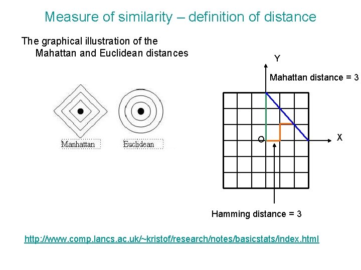
Measure of similarity – definition of distance The graphical illustration of the Mahattan and Euclidean distances Y Mahattan distance = 3 O Hamming distance = 3 http: //www. comp. lancs. ac. uk/~kristof/research/notes/basicstats/index. html X

Measure of similarity – definition of distance The higher the value of p, the more significant is the contribution of the largest components |ai – bi |. Close to 3, that is 3. 037 < 3. 162 Close to 10

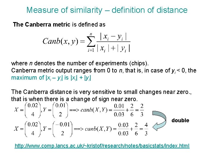
Measure of similarity – definition of distance The Canberra metric is defined as where n denotes the number of experiments (chips). Canberra metric output ranges from 0 to n, that is, in case of yi < 0, the maximum of |xi – yi| is |xi| + |yi| The Canberra distance is very sensitive to small changes near zero. , that is when there is a change of sign near zero. double http: //www. comp. lancs. ac. uk/~kristof/research/notes/basicstats/index. html

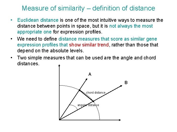
Measure of similarity – definition of distance • Euclidean distance is one of the most intuitive ways to measure the distance between points in space, but it is not always the most appropriate one for expression profiles. • We need to define distance measures that score as similar gene expression profiles that show similar trend, rather than those that depend on the absolute levels. • Two simple measures that can be used are the angle and chord distances. A B chord distance angular distance

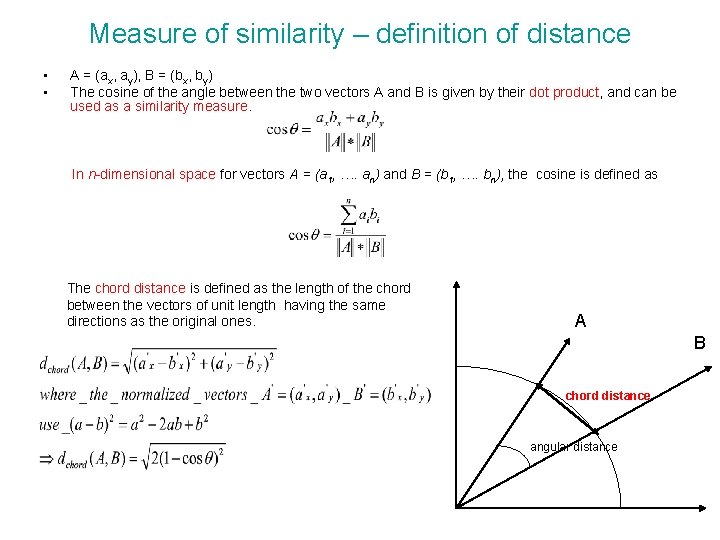
Measure of similarity – definition of distance • • A = (ax, ay), B = (bx, by) The cosine of the angle between the two vectors A and B is given by their dot product, and can be used as a similarity measure. In n-dimensional space for vectors A = (a 1, …. an) and B = (b 1, …. bn), the cosine is defined as The chord distance is defined as the length of the chord between the vectors of unit length having the same directions as the original ones. A B chord distance angular distance

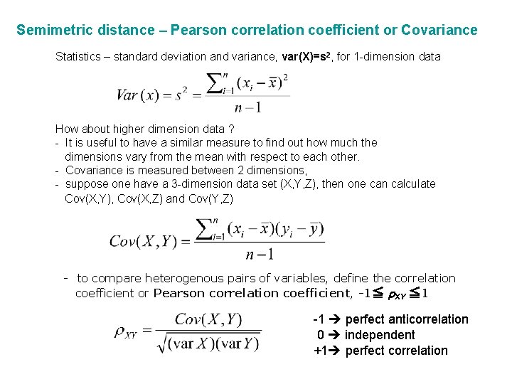
Semimetric distance – Pearson correlation coefficient or Covariance Statistics – standard deviation and variance, var(X)=s 2, for 1 -dimension data How about higher dimension data ? - It is useful to have a similar measure to find out how much the dimensions vary from the mean with respect to each other. - Covariance is measured between 2 dimensions, - suppose one have a 3 -dimension data set (X, Y, Z), then one can calculate Cov(X, Y), Cov(X, Z) and Cov(Y, Z) - to compare heterogenous pairs of variables, define the correlation coefficient or Pearson correlation coefficient, -1≦ r. XY ≦ 1 -1 perfect anticorrelation 0 independent +1 perfect correlation

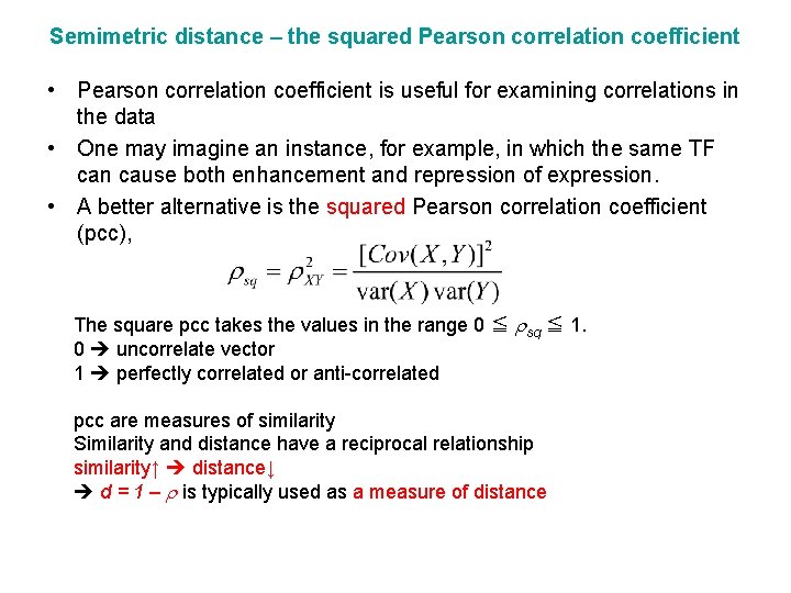
Semimetric distance – the squared Pearson correlation coefficient • Pearson correlation coefficient is useful for examining correlations in the data • One may imagine an instance, for example, in which the same TF can cause both enhancement and repression of expression. • A better alternative is the squared Pearson correlation coefficient (pcc), The square pcc takes the values in the range 0 ≦ rsq ≦ 1. 0 uncorrelate vector 1 perfectly correlated or anti-correlated pcc are measures of similarity Similarity and distance have a reciprocal relationship similarity↑ distance↓ d = 1 – r is typically used as a measure of distance

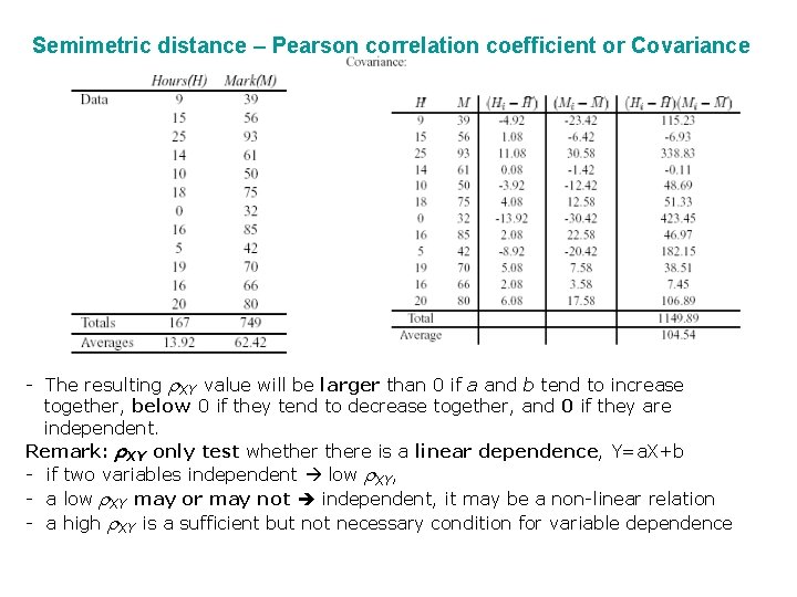
Semimetric distance – Pearson correlation coefficient or Covariance - The resulting r. XY value will be larger than 0 if a and b tend to increase together, below 0 if they tend to decrease together, and 0 if they are independent. Remark: r. XY only test whethere is a linear dependence, Y=a. X+b - if two variables independent low r. XY, - a low r. XY may or may not independent, it may be a non-linear relation - a high r. XY is a sufficient but not necessary condition for variable dependence

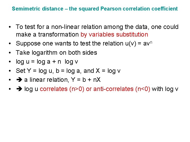
Semimetric distance – the squared Pearson correlation coefficient • To test for a non-linear relation among the data, one could make a transformation by variables substitution • Suppose one wants to test the relation u(v) = avn • Take logarithm on both sides • log u = log a + n log v • Set Y = log u, b = log a, and X = log v • a linear relation, Y = b + n. X • log u correlates (n>0) or anti-correlates (n<0) with log v

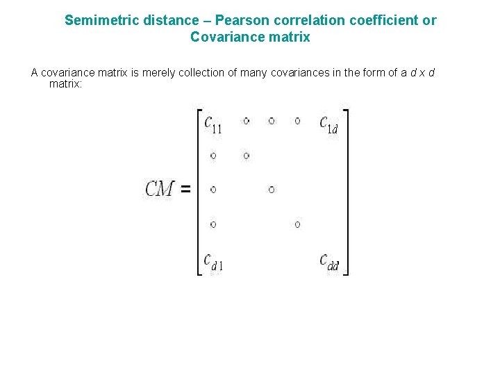
Semimetric distance – Pearson correlation coefficient or Covariance matrix A covariance matrix is merely collection of many covariances in the form of a d x d matrix:

Spearman’s rank correlation • One of the problems with using the PCC is that it is susceptible to being skewed by outliers: a single data point can result in two genes appearing to be correlated, even when all the other data points suggest that they are not. • Spearman’s rank correlation (SRC) is a non-parametric measure of correlation that is robust to outliers. • SRC is a measure that ignores the magnitude of the changes. The idea of the rank correlation is to transform the original values into ranks, and then to compute the correlation between the series of ranks. • First we order the values of gene A and B in ascending order, and assign the lowest value with rank 1. The SRC between A and B is defined as the PCC between ranked A and B. • In case of ties assign midranks both are ranked 5, then assign a rank of 5. 5

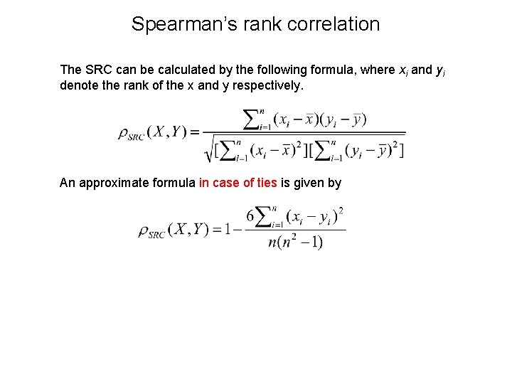
Spearman’s rank correlation The SRC can be calculated by the following formula, where xi and yi denote the rank of the x and y respectively. An approximate formula in case of ties is given by

Distances in discretized space • Sometimes it is advantageous to use a discreteized expression matrix as the starting point, e. g. to assign values 0 (expression unchanged, 1 (expression increased) and -1 (expression decreased). • The similarity between two discretized vectors can be measured by the notion of Shannon entropy.

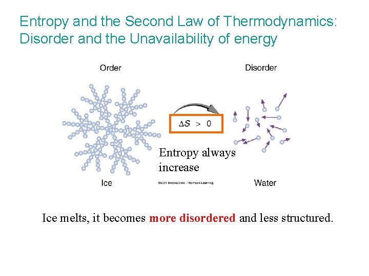
Entropy and the Second Law of Thermodynamics: Disorder and the Unavailability of energy Entropy always increase Ice melts, it becomes more disordered and less structured.

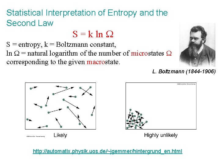
Statistical Interpretation of Entropy and the Second Law S = k ln W S = entropy, k = Boltzmann constant, ln W = natural logarithm of the number of microstates W corresponding to the given macrostate. L. Boltzmann (1844 -1906) http: //automatix. physik. uos. de/~jgemmer/hintergrund_en. html

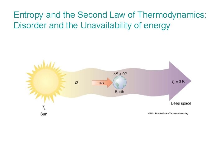
Entropy and the Second Law of Thermodynamics: Disorder and the Unavailability of energy

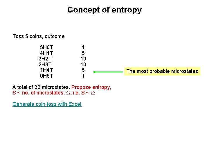
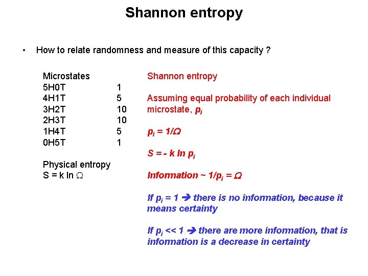
Concept of entropy Toss 5 coins, outcome 5 H 0 T 4 H 1 T 3 H 2 T 2 H 3 T 1 H 4 T 0 H 5 T 1 5 10 10 5 1 A total of 32 microstates. Propose entropy, S ~ no. of microstates, W, i. e. S ~ W Generate coin toss with Excel The most probable microstates

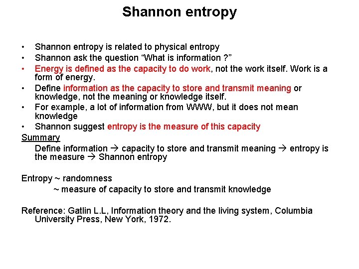
Shannon entropy • • • Shannon entropy is related to physical entropy Shannon ask the question “What is information ? ” Energy is defined as the capacity to do work, not the work itself. Work is a form of energy. • Define information as the capacity to store and transmit meaning or knowledge, not the meaning or knowledge itself. • For example, a lot of information from WWW, but it does not mean knowledge • Shannon suggest entropy is the measure of this capacity Summary Define information capacity to store and transmit meaning entropy is the measure Shannon entropy Entropy ~ randomness ~ measure of capacity to store and transmit knowledge Reference: Gatlin L. L, Information theory and the living system, Columbia University Press, New York, 1972.

Shannon entropy • How to relate randomness and measure of this capacity ? Microstates 5 H 0 T 4 H 1 T 3 H 2 T 2 H 3 T 1 H 4 T 0 H 5 T Physical entropy S = k ln W Shannon entropy 1 5 10 10 5 1 Assuming equal probability of each individual microstate, pi pi = 1/W S = - k ln pi Information ~ 1/pi = W If pi = 1 there is no information, because it means certainty If pi << 1 there are more information, that is information is a decrease in certainty

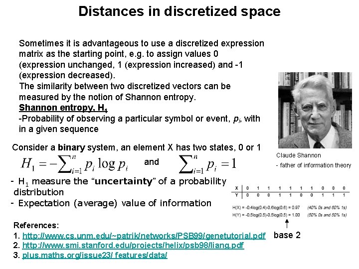
Distances in discretized space Sometimes it is advantageous to use a discretized expression matrix as the starting point, e. g. to assign values 0 (expression unchanged, 1 (expression increased) and -1 (expression decreased). The similarity between two discretized vectors can be measured by the notion of Shannon entropy, H 1 -Probability of observing a particular symbol or event, pi, with in a given sequence Consider a binary system, an element X has two states, 0 or 1 and Claude Shannon - father of information theory - H 1 measure the “uncertainty” of a probability distribution - Expectation (average) value of information References: 1. http: //www. cs. unm. edu/~patrik/networks/PSB 99/genetutorial. pdf 2. http: //www. smi. stanford. edu/projects/helix/psb 98/liang. pdf 3. plus. maths. org/issue 23/ features/data/ base 2

Shannon Entropy pi certain Uniform probability -1*1[log 2(1)] = 0 No information ½, ½ -2*1/2[log 2 (1/2)]=1 Maximal value 22 -states, 1/4 -4*1/4[log 2(1/4)]=2 1, 0 2 N-states, 1/2 N -2 N*1/2 N[log 2(2 N)]=N DNA seq. n = 4 states, maximum H 1 = - 4*(1/4)* log(1/4) = 2 bits Protein seq. n = 20 states, maximum = - 20*(1/20)*log(1/20) = 4. 322 bits, which is between 4 and 5 bits.

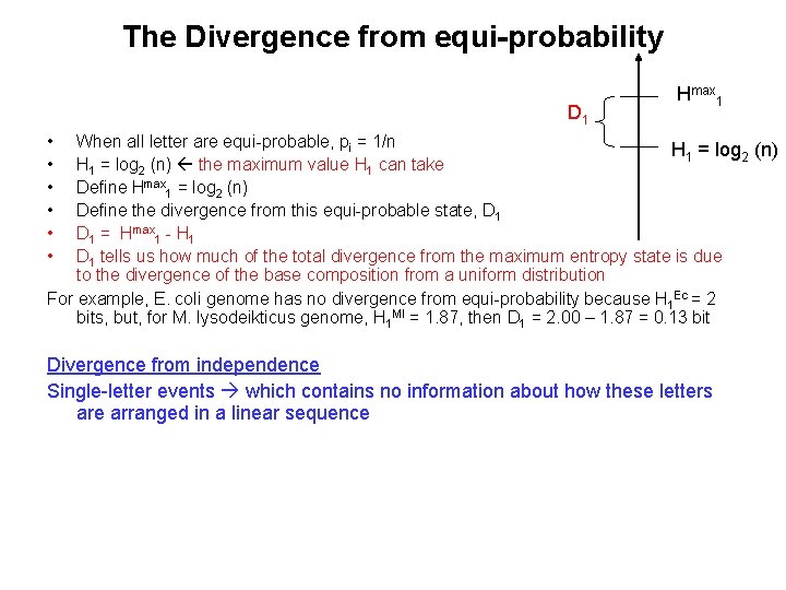
The Divergence from equi-probability D 1 Hmax 1 • • • When all letter are equi-probable, pi = 1/n H 1 = log 2 (n) the maximum value H 1 can take Define Hmax 1 = log 2 (n) Define the divergence from this equi-probable state, D 1 = Hmax 1 - H 1 D 1 tells us how much of the total divergence from the maximum entropy state is due to the divergence of the base composition from a uniform distribution For example, E. coli genome has no divergence from equi-probability because H 1 Ec = 2 bits, but, for M. lysodeikticus genome, H 1 Ml = 1. 87, then D 1 = 2. 00 – 1. 87 = 0. 13 bit Divergence from independence Single-letter events which contains no information about how these letters are arranged in a linear sequence

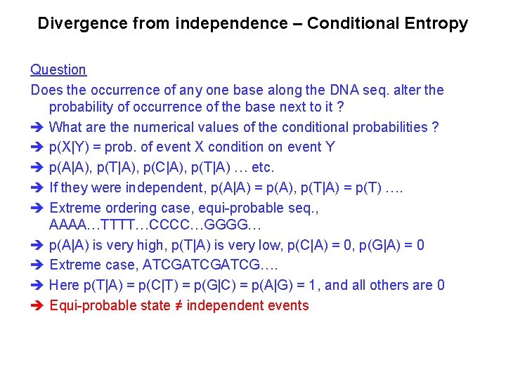
Divergence from independence – Conditional Entropy Question Does the occurrence of any one base along the DNA seq. alter the probability of occurrence of the base next to it ? What are the numerical values of the conditional probabilities ? p(X|Y) = prob. of event X condition on event Y p(A|A), p(T|A), p(C|A), p(T|A) … etc. If they were independent, p(A|A) = p(A), p(T|A) = p(T) …. Extreme ordering case, equi-probable seq. , AAAA…TTTT…CCCC…GGGG… p(A|A) is very high, p(T|A) is very low, p(C|A) = 0, p(G|A) = 0 Extreme case, ATCGATCG…. Here p(T|A) = p(C|T) = p(G|C) = p(A|G) = 1, and all others are 0 Equi-probable state ≠ independent events

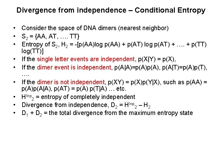
Divergence from independence – Conditional Entropy • Consider the space of DNA dimers (nearest neighbor) • S 2 = {AA, AT, …. TT} • Entropy of S 2, H 2 = -[p(AA)log p(AA) + p(AT) log p(AT) + …. + p(TT) log(TT)] • If the single letter events are independent, p(X|Y) = p(X), • If the dimer event is independent, p(A|A)=p(A), p(A|T)=p(A)p(T), …. • If the dimer is not independent, p(XY) = p(X)p(Y|X), such as p(AA) = p(A)p(A|A), p(AT) = p(A) p(T|A) … etc. • HInp 2 = entropy of completely independent • Divergence from independence, D 2 = HInp 2 – H 2 • D 1 + D 2 = the total divergence from the maximum entropy state

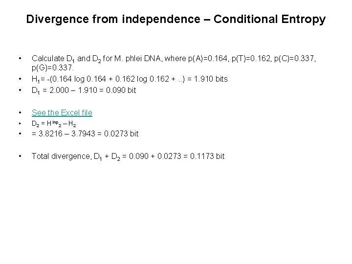
Divergence from independence – Conditional Entropy • • • Calculate D 1 and D 2 for M. phlei DNA, where p(A)=0. 164, p(T)=0. 162, p(C)=0. 337, p(G)=0. 337. H 1= -(0. 164 log 0. 164 + 0. 162 log 0. 162 +. . ) = 1. 910 bits D 1 = 2. 000 – 1. 910 = 0. 090 bit • See the Excel file • D 2 = HInp 2 – H 2 • = 3. 8216 – 3. 7943 = 0. 0273 bit • Total divergence, D 1 + D 2 = 0. 090 + 0. 0273 = 0. 1173 bit

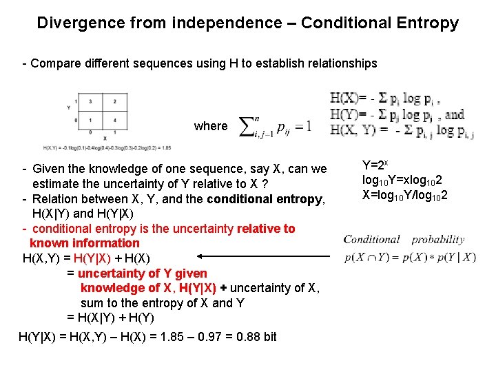
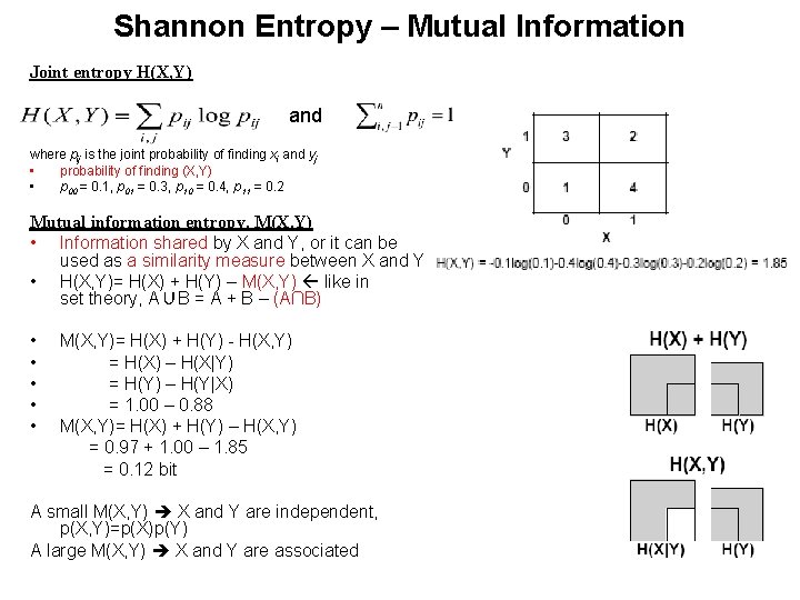
Divergence from independence – Conditional Entropy - Compare different sequences using H to establish relationships where - Given the knowledge of one sequence, say X, can we estimate the uncertainty of Y relative to X ? - Relation between X, Y, and the conditional entropy, H(X|Y) and H(Y|X) - conditional entropy is the uncertainty relative to known information H(X, Y) = H(Y|X) + H(X) = uncertainty of Y given knowledge of X, H(Y|X) + uncertainty of X, sum to the entropy of X and Y = H(X|Y) + H(Y) H(Y|X) = H(X, Y) – H(X) = 1. 85 – 0. 97 = 0. 88 bit Y=2 x log 10 Y=xlog 102 X=log 10 Y/log 102

Shannon Entropy – Mutual Information Joint entropy H(X, Y) and where pij is the joint probability of finding xi and yj • probability of finding (X, Y) • p 00 = 0. 1, p 01 = 0. 3, p 10 = 0. 4, p 11 = 0. 2 Mutual information entropy, M(X, Y) • Information shared by X and Y, or it can be used as a similarity measure between X and Y • H(X, Y)= H(X) + H(Y) – M(X, Y) like in set theory, A∪B = A + B – (A∩B) • • • M(X, Y)= H(X) + H(Y) - H(X, Y) = H(X) – H(X|Y) = H(Y) – H(Y|X) = 1. 00 – 0. 88 M(X, Y)= H(X) + H(Y) – H(X, Y) = 0. 97 + 1. 00 – 1. 85 = 0. 12 bit A small M(X, Y) X and Y are independent, p(X, Y)=p(X)p(Y) A large M(X, Y) X and Y are associated

Statistical Analysis of Microarray Data

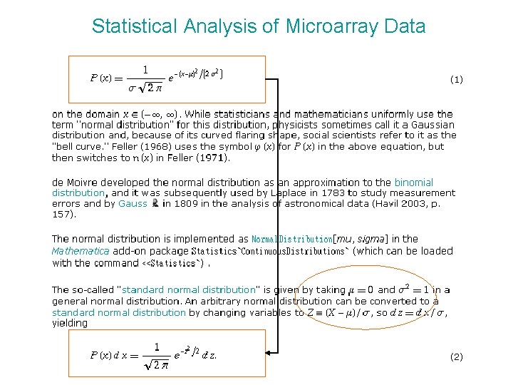
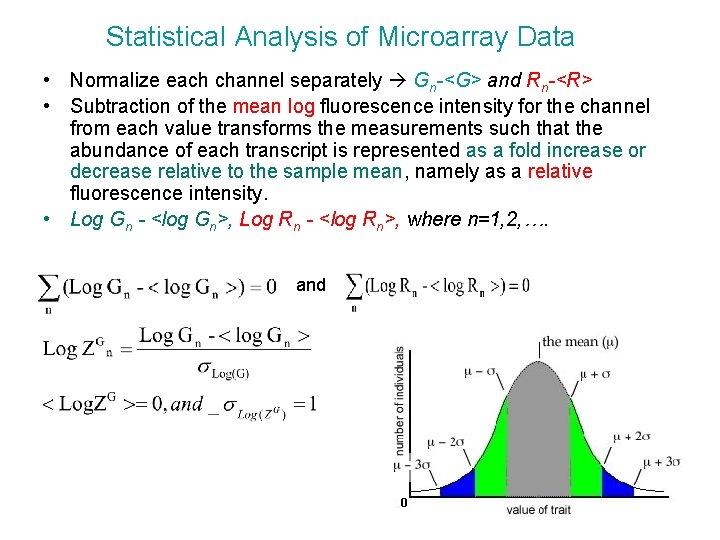
Statistical Analysis of Microarray Data • Normalize each channel separately Gn-<G> and Rn-<R> • Subtraction of the mean log fluorescence intensity for the channel from each value transforms the measurements such that the abundance of each transcript is represented as a fold increase or decrease relative to the sample mean, namely as a relative fluorescence intensity. • Log Gn - <log Gn>, Log Rn - <log Rn>, where n=1, 2, …. and

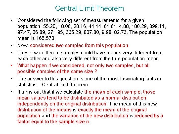
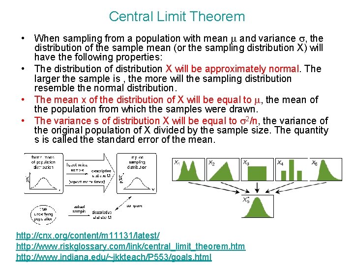
Central Limit Theorem • Considered the following set of measurements for a given population: 55. 20, 18. 06, 28. 16, 44. 14, 61. 61, 4. 88, 180. 29, 399. 11, 97. 47, 56. 89, 271. 95, 365. 29, 807. 80, 9. 98, 82. 73. The population mean is 165. 570. • Now, considered two samples from this population. • These two different samples could have means very different from each other and also very different from the true population mean. • What happen if we considered, not only two samples, but all possible samples of the same size ? • The answer to this question is one of the most fascinating facts in statistics – Central limit theorem. • It turns out that if we calculate the mean of each sample, those mean values tend to be distributed as a normal distribution, independently on the original distribution. The mean of this new distribution of the means is exactly the mean of the original population and the variance of the new distribution is reduced by a factor equal to the sample size n.

Central Limit Theorem • When sampling from a population with mean m and variance s, the distribution of the sample mean (or the sampling distribution X) will have the following properties: • The distribution of distribution X will be approximately normal. The larger the sample is , the more will the sampling distribution resemble the normal distribution. • The mean x of the distribution of X will be equal to m, the mean of the population from which the samples were drawn. • The variance s of distribution X will be equal to s 2/n, the variance of the original population of X divided by the sample size. The quantity s is called the standard error of the mean. http: //cnx. org/content/m 11131/latest/ http: //www. riskglossary. com/link/central_limit_theorem. htm http: //www. indiana. edu/~jkkteach/P 553/goals. html

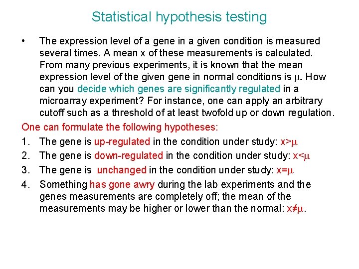
Statistical hypothesis testing • The expression level of a gene in a given condition is measured several times. A mean x of these measurements is calculated. From many previous experiments, it is known that the mean expression level of the given gene in normal conditions is m. How can you decide which genes are significantly regulated in a microarray experiment? For instance, one can apply an arbitrary cutoff such as a threshold of at least twofold up or down regulation. One can formulate the following hypotheses: 1. The gene is up-regulated in the condition under study: x>m 2. The gene is down-regulated in the condition under study: x<m 3. The gene is unchanged in the condition under study: x=m 4. Something has gone awry during the lab experiments and the genes measurements are completely off; the mean of the measurements may be higher or lower than the normal: x≠m.

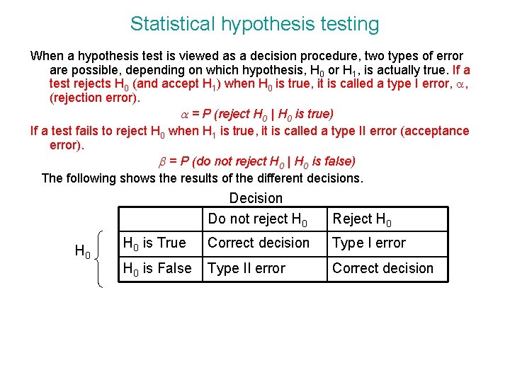
Statistical hypothesis testing When a hypothesis test is viewed as a decision procedure, two types of error are possible, depending on which hypothesis, H 0 or H 1, is actually true. If a test rejects H 0 (and accept H 1) when H 0 is true, it is called a type I error, a, (rejection error). a = P (reject H 0 | H 0 is true) If a test fails to reject H 0 when H 1 is true, it is called a type II error (acceptance error). b = P (do not reject H 0 | H 0 is false) The following shows the results of the different decisions. H 0 Decision Do not reject H 0 Reject H 0 is True Correct decision Type I error H 0 is False Type II error Correct decision

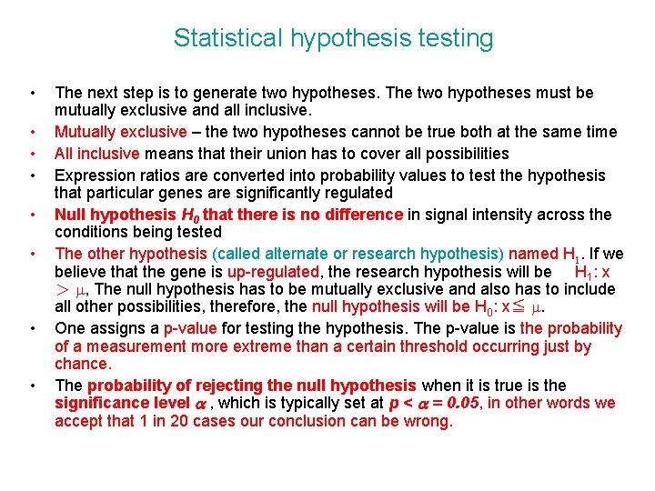
Statistical hypothesis testing • • The next step is to generate two hypotheses. The two hypotheses must be mutually exclusive and all inclusive. Mutually exclusive – the two hypotheses cannot be true both at the same time All inclusive means that their union has to cover all possibilities Expression ratios are converted into probability values to test the hypothesis that particular genes are significantly regulated Null hypothesis H 0 that there is no difference in signal intensity across the conditions being tested The other hypothesis (called alternate or research hypothesis) named H 1. If we believe that the gene is up-regulated, the research hypothesis will be H 1: x ＞ m, The null hypothesis has to be mutually exclusive and also has to include all other possibilities, therefore, the null hypothesis will be H 0: x≦ m. One assigns a p-value for testing the hypothesis. The p-value is the probability of a measurement more extreme than a certain threshold occurring just by chance. The probability of rejecting the null hypothesis when it is true is the significance level a , which is typically set at p < a = 0. 05, in other words we accept that 1 in 20 cases our conclusion can be wrong.

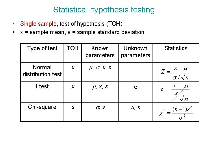
Statistical hypothesis testing • Single sample, test of hypothesis (TOH) • x = sample mean, s = sample standard deviation Type of test TOH Known parameters Unknown parameters Normal distribution test x m, s, x, s t-test x m, x, s s Chi-square s s, s m, x Statistics

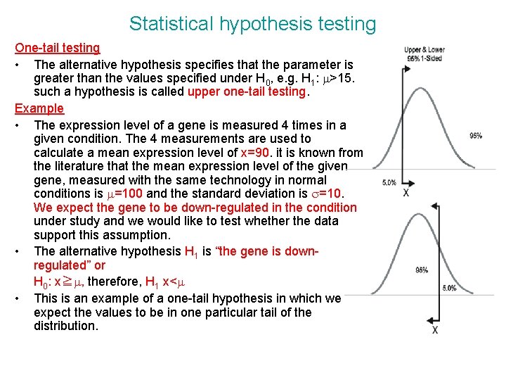
Statistical hypothesis testing One-tail testing • The alternative hypothesis specifies that the parameter is greater than the values specified under H 0, e. g. H 1: m>15. such a hypothesis is called upper one-tail testing. Example • The expression level of a gene is measured 4 times in a given condition. The 4 measurements are used to calculate a mean expression level of x=90. it is known from the literature that the mean expression level of the given gene, measured with the same technology in normal conditions is m=100 and the standard deviation is s=10. We expect the gene to be down-regulated in the condition under study and we would like to test whether the data support this assumption. • The alternative hypothesis H 1 is “the gene is downregulated” or H 0: x≧m, therefore, H 1 x<m • This is an example of a one-tail hypothesis in which we expect the values to be in one particular tail of the distribution.

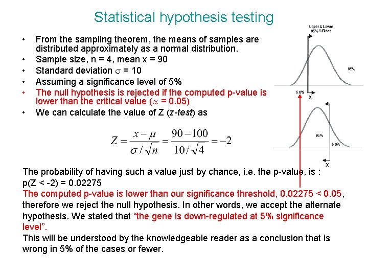
Statistical hypothesis testing • • • From the sampling theorem, the means of samples are distributed approximately as a normal distribution. Sample size, n = 4, mean x = 90 Standard deviation s = 10 Assuming a significance level of 5% The null hypothesis is rejected if the computed p-value is lower than the critical value (a = 0. 05) We can calculate the value of Z (z-test) as The probability of having such a value just by chance, i. e. the p-value, is : p(Z < -2) = 0. 02275 The computed p-value is lower than our significance threshold, 0. 02275 < 0. 05, therefore we reject the null hypothesis. In other words, we accept the alternate hypothesis. We stated that “the gene is down-regulated at 5% significance level”. This will be understood by the knowledgeable reader as a conclusion that is wrong in 5% of the cases or fewer.

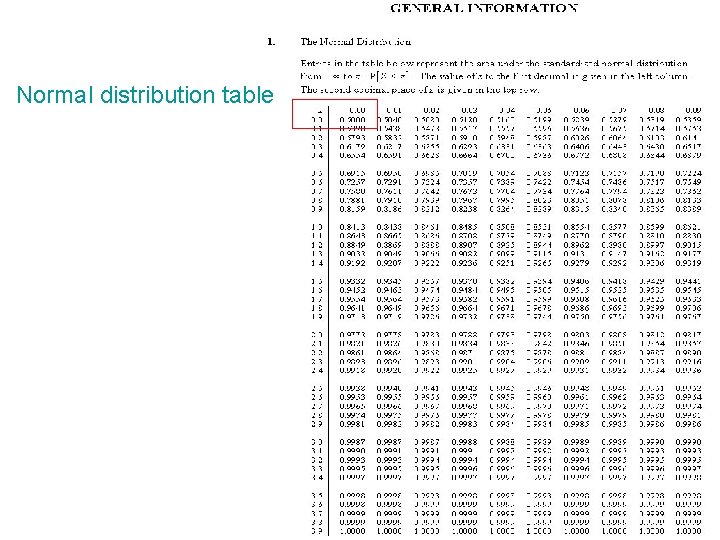
Normal distribution table

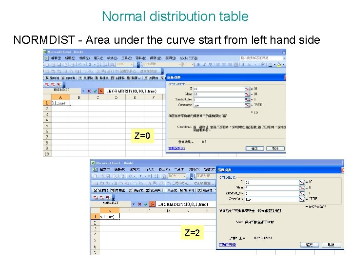
Normal distribution table NORMDIST - Area under the curve start from left hand side Z=0 Z=2

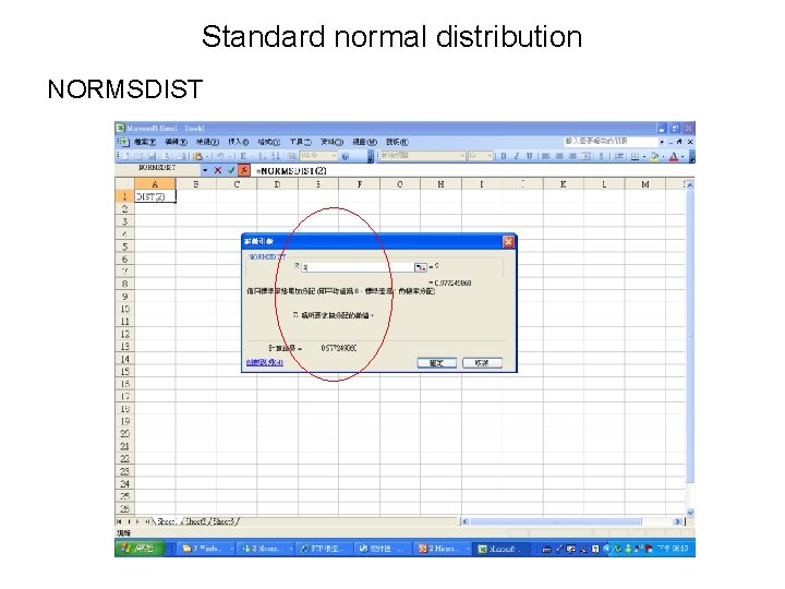
Standard normal distribution NORMSDIST

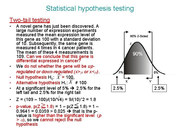
Statistical hypothesis testing Two-tail testing • • • A novel gene has just been discovered. A large number of expression experiments measured the mean expression level of this gene as 100 with a standard deviation of 10. Subsequently, the same gene is measured 4 times in 4 cancer patients. The mean of these 4 measurements is 109. Can we conclude that this gene is differential expressed in cancer? We do not whether the gene will be upregulated or down-regulated (x>m or x<m). Null hypothesis H 0: = 100, Alternative hypothesis H 1: ≠ 100 At a significant level of 5% 2. 5% for the left tail and 2. 5% for the right tail • Z = (109 – 100)/(10/√ 4) = 9/(10)*2 = 1. 8 • p-value, p(Z≧ 1. 8) = 1 – p(Z≦ 1. 8) = 1 – 0. 9641 = 0. 0359 > 0. 025 that is the pvalue is higher than the significant level (p > a), so we cannot reject the null hypothesis 2. 5%

Tests involving the mean – the t distribution • Hypothesis testing • Parametric testing – where the data are known or assumed to follow a certain probability distribution (e. g. normal distribution) • Non-parametric testing – where no a priori knowledge is available (do not know the underlying pdf, also called distribution free methods) and no such assumptions are made. • The t distribution test or student’s t distribution test is a parametric test, it was discovered by William S. Gossett, a 32 -year old research chemist employed by the famous Irish brewery (釀造，如啤酒) Guinness.

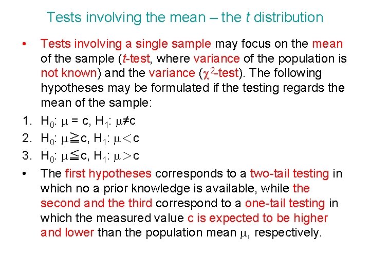
Tests involving the mean – the t distribution • Tests involving a single sample may focus on the mean of the sample (t-test, where variance of the population is not known) and the variance (c 2 -test). The following hypotheses may be formulated if the testing regards the mean of the sample: 1. H 0: m = c, H 1: m≠c 2. H 0: m≧c, H 1: m＜c 3. H 0: m≦c, H 1: m＞c • The first hypotheses corresponds to a two-tail testing in which no a prior knowledge is available, while the second and the third correspond to a one-tail testing in which the measured value c is expected to be higher and lower than the population mean m, respectively.

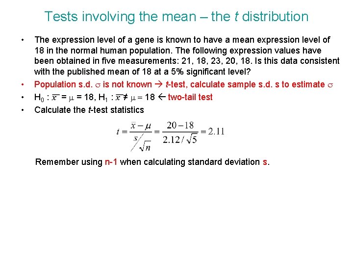
Tests involving the mean – the t distribution • • The expression level of a gene is known to have a mean expression level of 18 in the normal human population. The following expression values have been obtained in five measurements: 21, 18, 23, 20, 18. Is this data consistent with the published mean of 18 at a 5% significant level? Population s. d. s is not known t-test, calculate sample s. d. s to estimate s H 0 : = m = 18, H 1 : ≠ m = 18 two-tail test Calculate the t-test statistics Remember using n-1 when calculating standard deviation s.

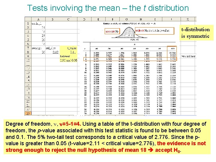
Tests involving the mean – the t distribution t-distribution is symmetric Degree of freedom, n, n=5 -1=4. Using a table of the t-distribution with four degree of freedom, the p-value associated with this test statistic is found to be between 0. 05 and 0. 1. The 5% two-tail test corresponds to a critical value of 2. 776. Since the pvalue is greater than 0. 05 (t-value=2. 11 < critical value=2. 776), the evidence is not strong enough to reject the null hypothesis of mean 18 accept H 0.

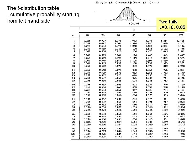
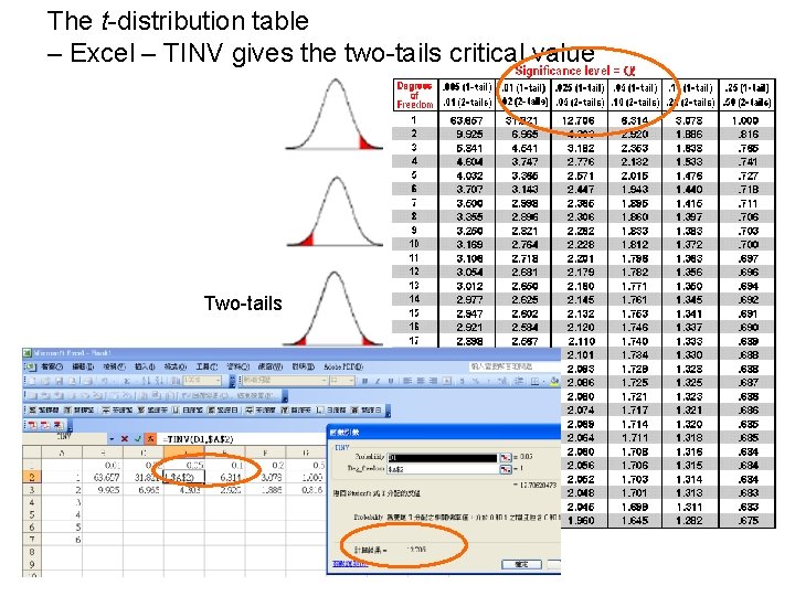
The t-distribution table - cumulative probability starting from left hand side Two-tails a=0. 10, 0. 05

The t-distribution table – Excel – TINV gives the two-tails critical value Two-tails

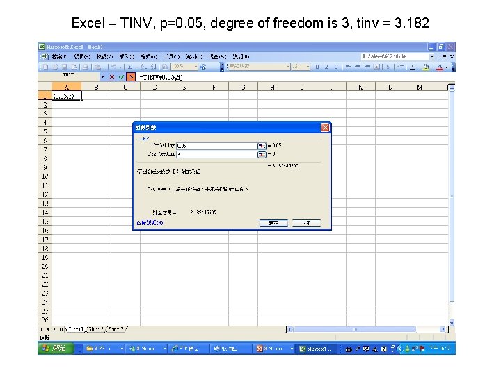
Excel – TINV, p=0. 05, degree of freedom is 3, tinv = 3. 182

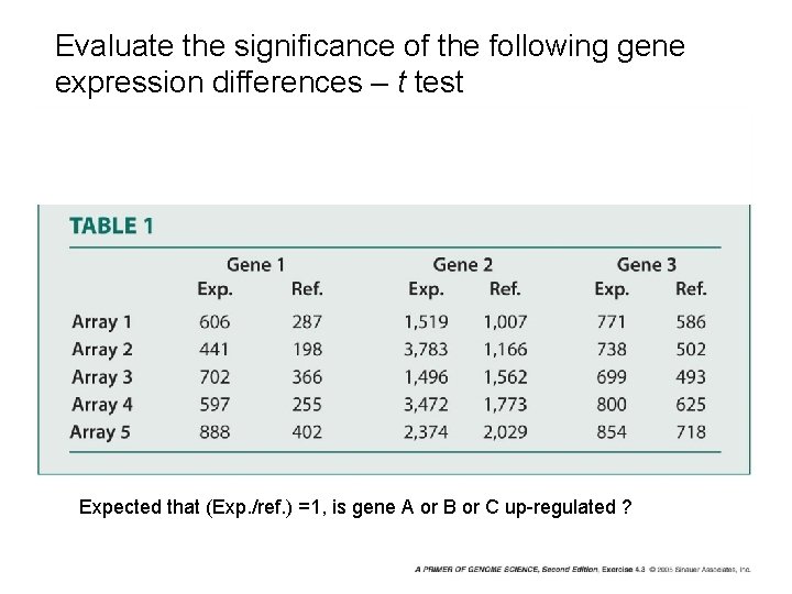
Evaluate the significance of the following gene expression differences – t test Expected that (Exp. /ref. ) =1, is gene A or B or C up-regulated ?

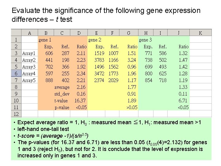
Evaluate the significance of the following gene expression differences – t test • • Expect average ratio = 1, H 0 : measured mean ≦ 1, H 1: measured mean >1 left-hand one-tail test t-score = (average -1)/(s/n 0. 5) The p-values (for 16. 37 and 6. 71) are less than 0. 05 (t 0. 05(4)=2. 132) for genes 1 and 3 (reject H 0), but not for 2. It is conclude that the level of expression is increased only in genes 1 and 3.

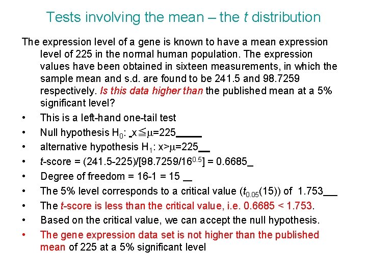
Tests involving the mean – the t distribution The expression level of a gene is known to have a mean expression level of 225 in the normal human population. The expression values have been obtained in sixteen measurements, in which the sample mean and s. d. are found to be 241. 5 and 98. 7259 respectively. Is this data higher than the published mean at a 5% significant level? • This is a left-hand one-tail test • Null hypothesis H 0: x≦m=225 • alternative hypothesis H 1: x>m=225 • t-score = (241. 5 -225)/[98. 7259/160. 5] = 0. 6685 • Degree of freedom = 16 -1 = 15 • The 5% level corresponds to a critical value (t 0. 05(15)) of 1. 753 • The t-score is less than the critical value, i. e. 0. 6685 < 1. 753. • Based on the critical value, we can accept the null hypothesis. • The gene expression data set is not higher than the published mean of 225 at a 5% significant level

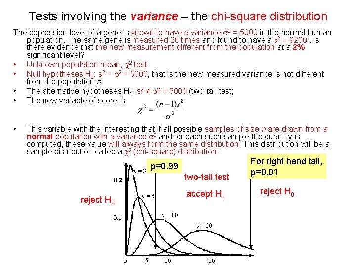
Tests involving the variance – the chi-square distribution The expression level of a gene is known to have a variance s 2 = 5000 in the normal human population. The same gene is measured 26 times and found to have a s 2 = 9200. Is there evidence that the new measurement different from the population at a 2% significant level? • Unknown population mean, c 2 test • Null hypotheses H 0: s 2 = 5000, that is the new measured variance is not different from the population s • The alternative hypotheses H 1: s 2 ≠ s 2 = 5000 (two-tail test) • The new variable of score is • This variable with the interesting that if all possible samples of size n are drawn from a normal population with a variance s 2 and for each such sample the quantity is computed, these value will always form the same distribution. This distribution will be a sample distribution called a c 2 (chi-square) distribution. p=0. 99 two-tail test reject H 0 accept H 0 For right hand tail, p=0. 01 reject H 0

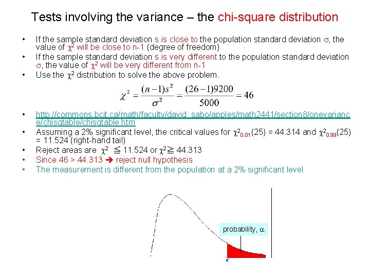
Tests involving the variance – the chi-square distribution • • If the sample standard deviation s is close to the population standard deviation s, the value of c 2 will be close to n-1 (degree of freedom) If the sample standard deviation s is very different to the population standard deviation s, the value of c 2 will be very different from n-1 Use the c 2 distribution to solve the above problem. http: //commons. bcit. ca/math/faculty/david_sabo/apples/math 2441/section 8/onevarianc e/chisqtable. htm Assuming a 2% significant level, the critical values for c 20. 01(25) = 44. 314 and c 20. 99(25) = 11. 524 (right-hand tail) Reject areas are c 2 ≦ 11. 524 or c 2≧ 44. 313 Since 46 > 44. 313 reject null hypothesis The measurement is different from the population at a 2% significant level probability, a

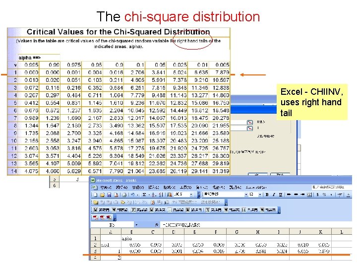
The chi-square distribution Excel - CHIINV, uses right hand tail

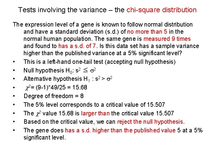
Tests involving the variance – the chi-square distribution The expression level of a gene is known to follow normal distribution and have a standard deviation (s. d. ) of no more than 5 in the normal human population. The same gene is measured 9 times and found to has a s. d. of 7. Is this data set has a sample variance higher than the published variance at a 5% significant level? • This is a left-hand one-tail test (accepting null hypothesis) • Null hypothesis H 0: s 2 ≦ s 2 • Alternative hypothesis H 1 : s 2 > s 2 • c 2= (9 -1)*49/25 = 15. 68 • Degree of freedom = 8 • The 5% level corresponds to a critical value of 15. 507 • The c 2 value 15. 68 is larger than the critical value 15. 507 • Based on the critical value, we can reject the null hypothesis. • The gene does has a s. d. higher than the published value 5 at a 5% significant level.

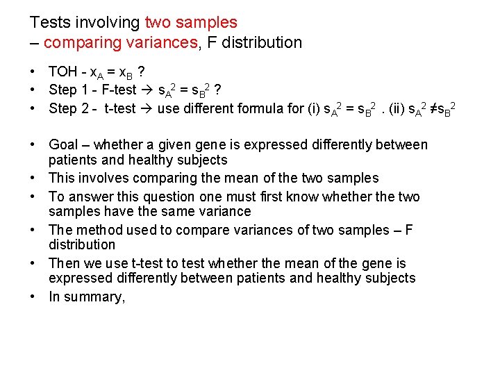
Tests involving two samples – comparing variances, F distribution • TOH - x. A = x. B ? • Step 1 - F-test s. A 2 = s. B 2 ? • Step 2 - t-test use different formula for (i) s. A 2 = s. B 2. (ii) s. A 2 ≠s. B 2 • Goal – whether a given gene is expressed differently between patients and healthy subjects • This involves comparing the mean of the two samples • To answer this question one must first know whether the two samples have the same variance • The method used to compare variances of two samples – F distribution • Then we use t-test to test whether the mean of the gene is expressed differently between patients and healthy subjects • In summary,

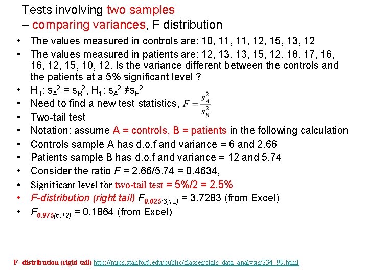
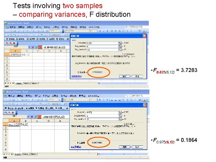
Tests involving two samples – comparing variances, F distribution • The values measured in controls are: 10, 11, 12, 15, 13, 12 • The values measured in patients are: 12, 13, 15, 12, 18, 17, 16, 12, 15, 10, 12. Is the variance different between the controls and the patients at a 5% significant level ? • H 0: s. A 2 = s. B 2, H 1: s. A 2 ≠s. B 2 • Need to find a new test statistics, • Two-tail test • Notation: assume A = controls, B = patients in the following calculation • Controls sample A has d. o. f and variance = 6 and 2. 66 • Patients sample B has d. o. f and variance = 12 and 5. 74 • Consider the ratio F = 2. 66/5. 74 = 0. 4634, • Significant level for two-tail test = 5%/2 = 2. 5% • F-distribution (right tail) F 0. 025(6, 12) = 3. 7283 (from Excel) • F 0. 975(6, 12) = 0. 1864 (from Excel) F- distribution (right tail) http: //mips. stanford. edu/public/classes/stats_data_analysis/234_99. html

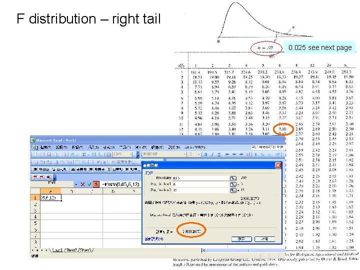
F distribution – right tail 0. 025 see next page

Tests involving two samples – comparing variances, F distribution • F 0. 025(6, 12) = 3. 7283 • F 0. 975(6, 12) = 0. 1864

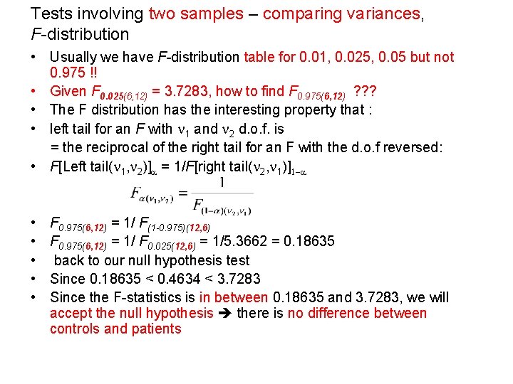
Tests involving two samples – comparing variances, F-distribution • Usually we have F-distribution table for 0. 01, 0. 025, 0. 05 but not 0. 975 !! • Given F 0. 025(6, 12) = 3. 7283, how to find F 0. 975(6, 12) ? ? ? • The F distribution has the interesting property that : • left tail for an F with n 1 and n 2 d. o. f. is = the reciprocal of the right tail for an F with the d. o. f reversed: • F[Left tail(n 1, n 2)]a = 1/F[right tail(n 2, n 1)]1 -a • • • F 0. 975(6, 12) = 1/ F(1 -0. 975)(12, 6) F 0. 975(6, 12) = 1/ F 0. 025(12, 6) = 1/5. 3662 = 0. 18635 back to our null hypothesis test Since 0. 18635 < 0. 4634 < 3. 7283 Since the F-statistics is in between 0. 18635 and 3. 7283, we will accept the null hypothesis there is no difference between controls and patients

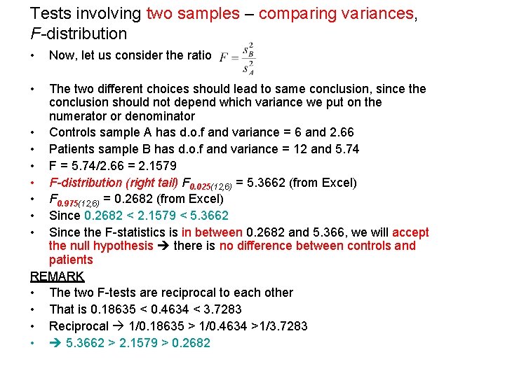
Tests involving two samples – comparing variances, F-distribution • • Now, let us consider the ratio The two different choices should lead to same conclusion, since the conclusion should not depend which variance we put on the numerator or denominator • Controls sample A has d. o. f and variance = 6 and 2. 66 • Patients sample B has d. o. f and variance = 12 and 5. 74 • F = 5. 74/2. 66 = 2. 1579 • F-distribution (right tail) F 0. 025(12, 6) = 5. 3662 (from Excel) • F 0. 975(12, 6) = 0. 2682 (from Excel) • Since 0. 2682 < 2. 1579 < 5. 3662 • Since the F-statistics is in between 0. 2682 and 5. 366, we will accept the null hypothesis there is no difference between controls and patients REMARK • The two F-tests are reciprocal to each other • That is 0. 18635 < 0. 4634 < 3. 7283 • Reciprocal 1/0. 18635 > 1/0. 4634 >1/3. 7283 • 5. 3662 > 2. 1579 > 0. 2682

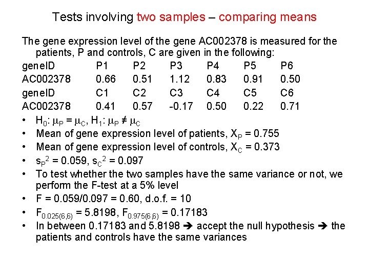
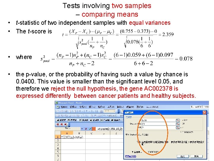
Tests involving two samples – comparing means The gene expression level of the gene AC 002378 is measured for the patients, P and controls, C are given in the following: gene. ID P 1 P 2 P 3 P 4 P 5 P 6 AC 002378 0. 66 0. 51 1. 12 0. 83 0. 91 0. 50 gene. ID C 1 C 2 C 3 C 4 C 5 C 6 AC 002378 0. 41 0. 57 -0. 17 0. 50 0. 22 0. 71 • H 0: m. P = m. C, H 1: m. P ≠ m. C • Mean of gene expression level of patients, XP = 0. 755 • Mean of gene expression level of controls, XC = 0. 373 • s. P 2 = 0. 059, s. C 2 = 0. 097 • To test whether the two samples have the same variance or not, we perform the F-test at a 5% level • F = 0. 059/0. 097 = 0. 60, d. o. f. = 10 • F 0. 025(6, 6) = 5. 8198, F 0. 975(6, 6) = 0. 17183 • In between 0. 17183 and 5. 8198 accept the null hypothesis the patients and controls have the same variances

Tests involving two samples – comparing means • t-statistic of two independent samples with equal variances • The t-score is • where • the p-value, or the probability of having such a value by chance is 0. 0400. This value is smaller than the significant level 0. 05, and therefore we reject the null hypothesis, the gene AC 002378 is expressed differently between cancer patients and healthy subjects.

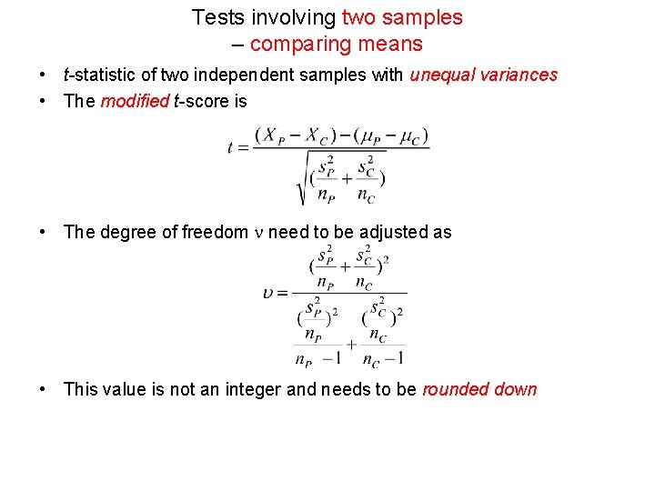
Tests involving two samples – comparing means • t-statistic of two independent samples with unequal variances • The modified t-score is • The degree of freedom n need to be adjusted as • This value is not an integer and needs to be rounded down

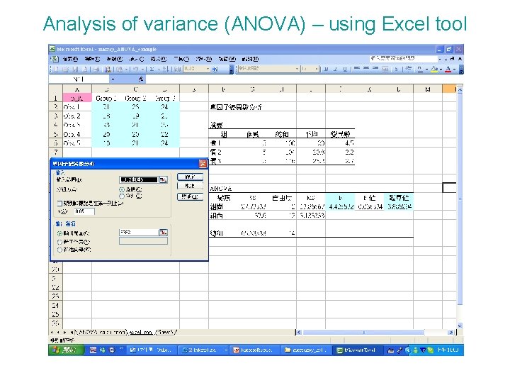
Analysis of variance (ANOVA) • How do we compare multiple samples at once? • We could do pairwise t-tests to see which differed from one another. • However, the a-level probability of making an error applies to each test. So, the real chance of making an error is increased by using multiple tests. • There are ways of dealing with this, but it is timeconsuming to do many pairs. • The analysis of variance procedure (called ANOVA) is a way to make multiple comparisons. • H 0 : m 1 = m 2 = m 3 =. . mn, for n means • Ha : at least one mean is not equal to the others, i. e. mi ≠ mj , or mj ≠ mk or mi ≠ mj ≠ mk or more http: //www. tnstate. edu/ganter/BIO%20311%20 Ch%2011%20 Many. Means. html

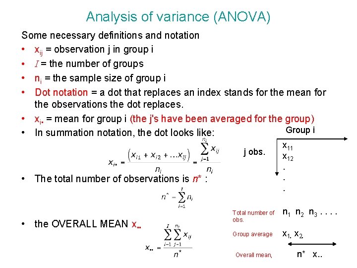
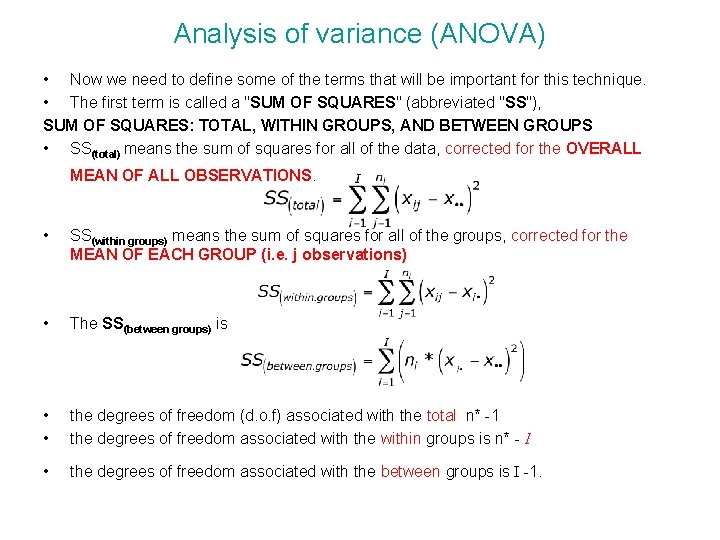
Analysis of variance (ANOVA) Some necessary definitions and notation • xij = observation j in group i • I = the number of groups • ni = the sample size of group i • Dot notation = a dot that replaces an index stands for the mean for the observations the dot replaces. • xi • = mean for group i (the j's have been averaged for the group) Group i • In summation notation, the dot looks like: j obs. • The total number of observations is n* : • the OVERALL MEAN x • • x 11 x 12. . . Total number of obs. n 1 n 2 n 3. . Group average x 1. x 2. Overall mean, n* x. .

Analysis of variance (ANOVA) • Now we need to define some of the terms that will be important for this technique. • The first term is called a "SUM OF SQUARES" (abbreviated "SS"), SUM OF SQUARES: TOTAL, WITHIN GROUPS, AND BETWEEN GROUPS • SS(total) means the sum of squares for all of the data, corrected for the OVERALL MEAN OF ALL OBSERVATIONS. • SS(within groups) means the sum of squares for all of the groups, corrected for the MEAN OF EACH GROUP (i. e. j observations) • The SS(between groups) is • • the degrees of freedom (d. o. f) associated with the total n* -1 the degrees of freedom associated with the within groups is n* - I • the degrees of freedom associated with the between groups is I -1.

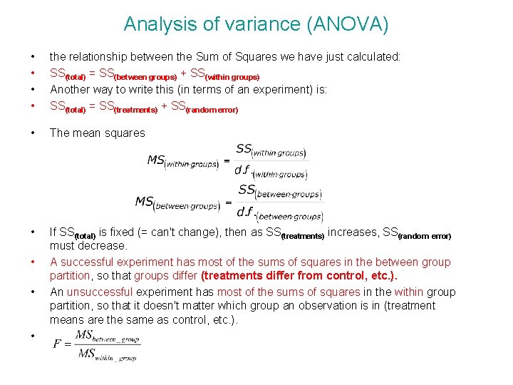
Analysis of variance (ANOVA) • • the relationship between the Sum of Squares we have just calculated: SS(total) = SS(between groups) + SS(within groups) Another way to write this (in terms of an experiment) is: SS(total) = SS(treatments) + SS(random error) • The mean squares • If SS(total) is fixed (= can't change), then as SS(treatments) increases, SS(random error) must decrease. A successful experiment has most of the sums of squares in the between group partition, so that groups differ (treatments differ from control, etc. ). An unsuccessful experiment has most of the sums of squares in the within group partition, so that it doesn't matter which group an observation is in (treatment means are the same as control, etc. ). • • •

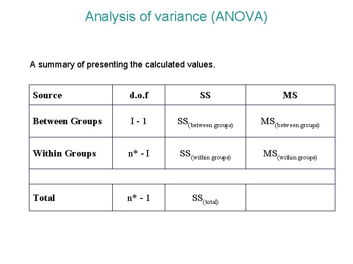
Analysis of variance (ANOVA) A summary of presenting the calculated values. Source d. o. f SS MS Between Groups I-1 SS(between groups) MS(between groups) Within Groups n* - I SS(within groups) MS(within groups) Total n* - 1 SS(total)

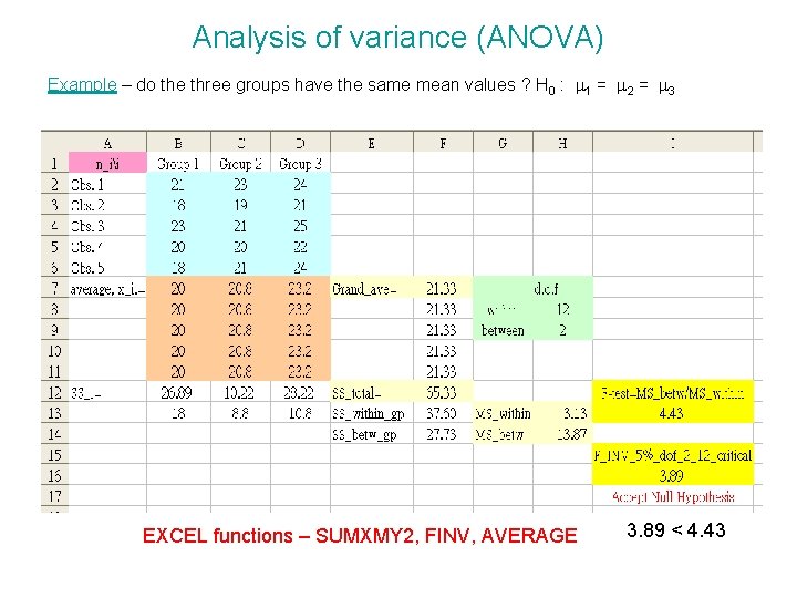
Analysis of variance (ANOVA) Example – do the three groups have the same mean values ? H 0 : m 1 = m 2 = m 3 EXCEL functions – SUMXMY 2, FINV, AVERAGE 3. 89 < 4. 43

Analysis of variance (ANOVA) – using Excel tool

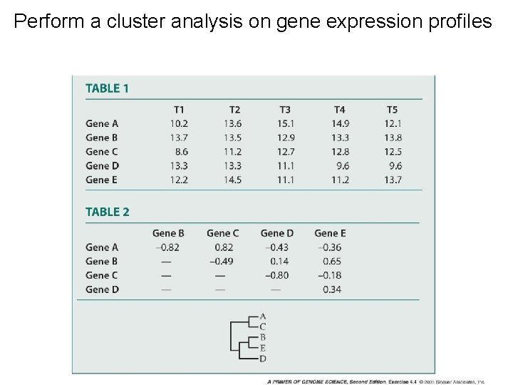
Perform a cluster analysis on gene expression profiles

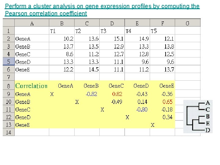
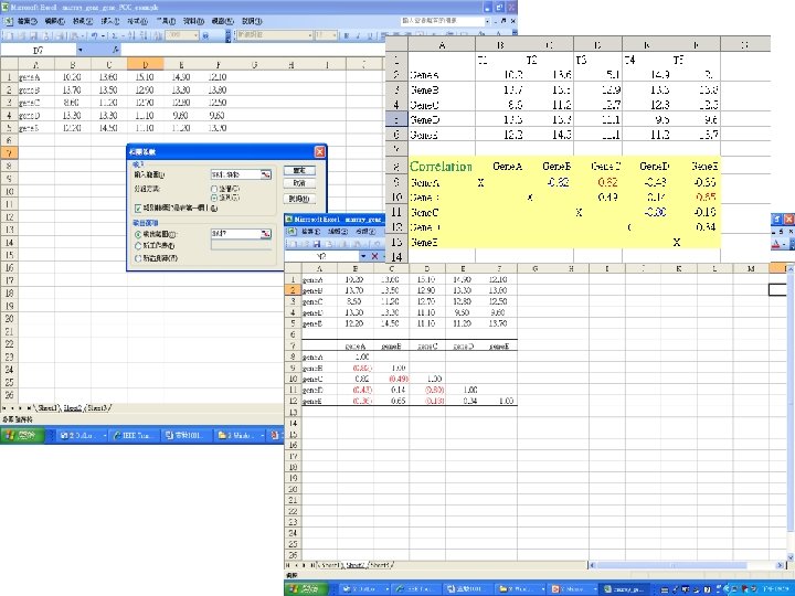
Perform a cluster analysis on gene expression profiles by computing the Pearson correlation coefficient

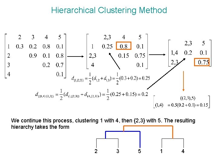
Hierarchical Clustering Method We continue this process, clustering 1 with 4, then {2, 3} with 5. The resulting hierarchy takes the form 2 3 5 1 4

References 1. Draghici S. Data analysis tools for DNA microarrays. Chapman & Hall/CRC 2003. 2. Gibson and Muse. A primer of Genome Science. 2 nd ed. Sinauer 2004. 3. Stekel D. Microarray Bioinformatics. Cambridge University Press 2003. 4. Tamhane and Dunlop Statistics and data analysis, from elementary to intermediate. Prentice Hall 2000.