Signals and Systems ANURAG GROUP OF INSTITUTION Signal

Signals and Systems ANURAG GROUP OF INSTITUTION

Signal is a set of data or information collected over time.

Signal Classification Signals may be classified into: 1. Continuous-time and discrete-time signals 2. Analogue and digital signals 3. Periodic and aperiodic signals 4. Energy and power signals 5. Deterministic and probabilistic signals 6. Causal and non-causal 7. Even and Odd signals

Signal Classification- Continuous vs Discrete Continuous-time Discrete-time

Signal Classification- Analogue vs Digital Analogue, continuous Analogue, discrete Digital, continuous Digital, discrete

Signal Classification- Periodic vs Aperiodic A signal x(t) is said to be periodic if for some positive constant To x(t) = x (t+To) for all t The smallest value of To that satisfies the periodicity condition of this equation is the fundamental period of x(t).

Signal Classification- Energy v/s Power • Energy of a signal x(t) is given by: • Power of a signal x(t) is given by: • A signal is Energy signal if • A signal is Power signal if

Signal Classification- Deterministic vs Random Deterministic Random

Signal Classification- Causal vs Non-causal

Signal Classification- Even vs Odd

Even and Odd Function Even and odd functions have the following properties: • Even x Odd = Odd • Odd x Odd = Even • Even x Even = Even Every signal x(t) can be expressed as a sum of even and odd components because:

Even and Odd Function Consider the causal exponential function

Signal Models – Unit Step Function u(t) Step function defined by: Useful to describe a signal that begins at t = 0 (i. e. causal signal). For example, the signal e-at represents an everlasting exponential that starts at t = -. The causal for of this exponential e-atu(t)

• Continuous Unit Impulse and Step Signals The continuous unit impulse signal is defined: • Note that it is discontinuous at t=0 • The arrow is used to denote area, rather than actual value • Again, useful for an infinite basis • The continuous unit step signal is defined:

Signal Models – Pulse Signal A pulse signal can be presented by two step functions: x(t) = u(t-2) – u(t-4)

Signal Models – Unit Impulse Function δ(t) First defined by Dirac as:

Multiplying Function (t) by an Impulse Since impulse is non-zero only at t = 0, and (t) at t = 0 is (0), we get: We can generalize this for t = T:

Sampling Property of Unit Impulse Function Since we have: It follows that: This is the same as “sampling” (t) at t = 0. If we want to sample (t) at t = T, we just multiple (t) with This is called the “sampling or sifting property” of the impulse.

Examples Simplify the following expression Evaluate the following Find dx/dt for the following signal x(t) = u(t-2) – 3 u(t-4)

The Complex Exponential Function est This exponential function is very important in signals & systems, and the parameter s is a complex variable given by:

The Complex Exponential Function est If = 0, then we have the function ejωt, which has a real frequency of ω Therefore the complex variable s = +jω is the complex frequency The function est can be used to describe a very large class of signals and functions. Here a number of example:

The Exponential Function est

The Complex Frequency Plane s= + jω A real function xe(t) is said to be an even function of t if A real function xo(t) is said to be an odd function of t if HW 1_Ch 1: 1. 1 -3, 1. 1 -4, 1. 2 -2(a, b, d), 1. 2 -5, 1. 4 -3, 1. 4 -4, 1. 4 -5, 1. 4 -10 (b, f)

• Unit gate function (a. k. a. unit pulse function) rect( 1 x) -1/2 0 1/2 x • What does rect(x / a) look like? • Unit triangle function D(x) 1 -1/2 0 1/2 x

• Sinc function sinc(x) 1 x -3 p -2 p -p 0 p 2 p 3 p – Even function – Zero crossings at – Amplitude decreases proportionally to 1/x

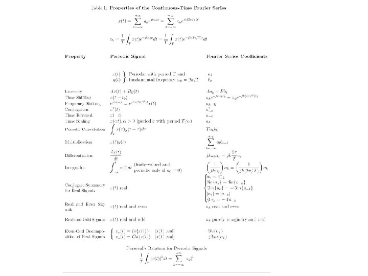
CONTENTS • • • Fourier Series Fourier Transforms Power and Energy Sampling of Bandlimited Signals Bandpass Signals

FOURIER SERIES • Usually, a signal is described as a function of time. • There are some amazing advantages if a signal can be expressed in the frequency domain. • Fourier transform analysis is named after Jean Baptiste Joseph Fourier (1768 -1830).

Fourier series (FS) is used for representing a continuoustime periodic signal as weighted superposition of sinusoids. Periodic Signals A continuous-time signal is said to be periodic if there exists a positive constant such that where T 0 is the period of the signal.

: fundamental Period : fundamental frequency Example: Periodic and aperiodic signal

• {xn} are called the Fourier series coefficients of the signal x(t). • The quantity is called the fundamental frequency of the signal x(t) • The Fourier series expansion can be expressed in terms of angular frequency by and

Example: Let x(t) denote the periodic signal depicted in Figure 2. 2 where is a rectangular pulse. Determine the Fourier series expansion for this signal.

Solution: We first observe that the period of the signal is T 0 and

Therefore, we have

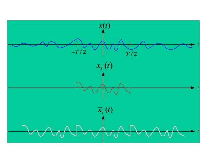
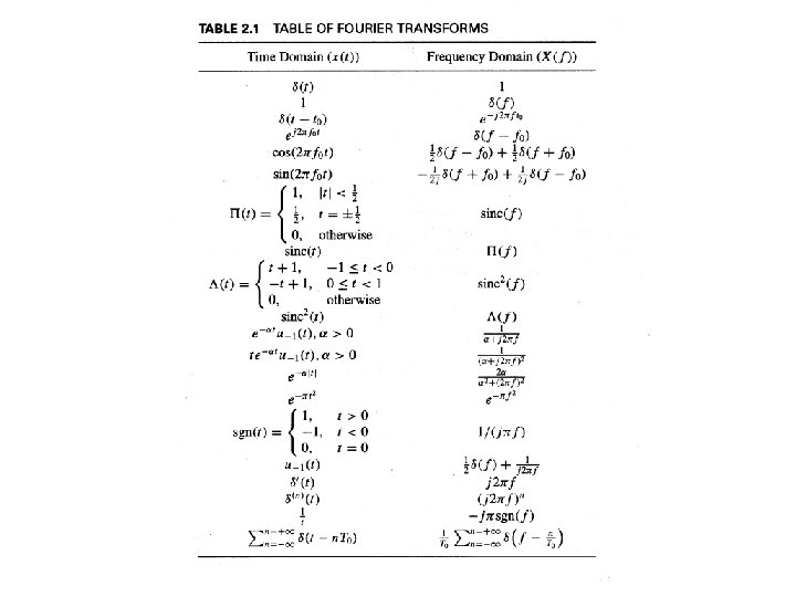
FOURIER TRANSFORMS • Fourier transform is the extension of Fourier series to periodic and aperiodic signals. • The signals are expressed in terms of complex exponentials of various frequencies, but these frequencies are not discrete. • The extension of the Fourier series to aperiodic signals can be done by extending the period to infinity. • The signal has a continuous spectrum as opposed to a discrete spectrum.

• Assume that the Fourier series of periodic extension of the nonperiodic signal exists. • Define as the truncation of over , i. e. ,

Denote the periodic signal Conversely, we may express the truncated signal by

• If we let the period T approach infinity, then in the limit, the periodic signal approximately becomes the aperiodic signal

• As far as the integration is concerned, the integrand on this integral can be rewritten as • Define • We have

• We have the Fourier series representation • Taking the limit, we obtain • As That is, in the limit, the frequency spacing becomes small.

• The summation turns to become an integral • is the inverse Fourier transform of . • The Fourier transform of x(t) is

• Definition III. Suppose that, is a signal such that it is absolutely integrable, that is, Then the Fourier transform of defined as is The inverse Fourier transform is given by

• Observations – X(f) is in general a complex function. The function X(f) is sometimes referred to as the spectrum of the signal x(t). – To denote that X(f) is the Fourier transform of x(t), the following notation is frequently employed – To denote that x(t) is the inverse Fourier transform of X(f) , the following notation is used – Sometimes the following notation is used as a shorthand for both relations

– The Fourier transform and the inverse Fourier transform relations can be written as On the other hand, where have is the unit impulse. From above equation, we may or, in general Hence, the spectrum of is equal to unity over all frequencies.

Example 2. 2. 1: Determine the Fourier transform of the signal. Solution: We have

• The Fourier transform of .

Example 2. 2. 2: Find the Fourier transform of the impulse signal. Solution: The Fourier transform can be obtained by Similarly, from the relation We conclude that

• The Fourier transform of .

2. 2. 2 Basic Properties of the Fourier Transform • Linearity Property: Given signals Fourier transforms The Fourier transform of and is with the

• Duality Property: Proof:

• Time Shift Property: A shift of in the time origin causes a phase shift of in the frequency domain. Proof: Let

• Scaling Property: For any real • Proof: Case 1: Let ; we have Case 2: Let ; we have , we have

• Convolution Property: If the signal possess Fourier transforms, then Proof: Convolution and both

• Modulation Property: The Fourier transform of is , and the Fourier transform of is Proof:

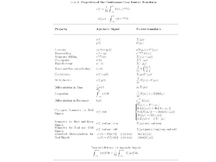
• Parseval’s Property: If the Fourier transforms of and are denoted by and , respectively, then

• proof:

• Rayleigh’s Property: If X(f) is the Fourier transform of x(t), then Proof: Parseval’s Property

• Autocorrelation Property: The (time) autocorrelation function of the aperiodic signal x(t) is denoted by and is defined by The autocorrelation property states that • Differentiation Property: The Fourier transform of the derivative of a signal can be obtained from the relation

• Integration Property: The Fourier transform of the integral of a signal can be determined from the relation • Moments Property: If , then , the nth moment of x(t), can be obtained from the relation

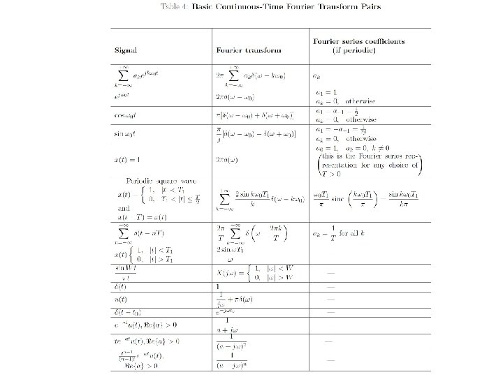
2. 2. 3 Fourier Transform for Periodic Signals • Let x(t) be a periodic signal with period. Let denote the Fourier series coefficients corresponding to this signal. Then • Since we obtain

• If we define the truncated signal we may have as

• By using the convolution theorem, we obtain Comparing this result with we conclude

• Alternative way to find the Fourier series coefficients. Given the periodic signal x(t), we carry out the following steps to find : 1. Find the truncated signal . 2. Determine the Fourier transform truncated signal. of the 3. Evaluate the Fourier transform of the truncated signal at , to obtain the nth harmonic and multiply by

• Example 2. 2. 3: Determine the Fourier series coefficients of the signal x(t) shown in Figure 2. 2. Solution: The truncated signal is and its Fourier transform is Therefore,

2. 3 POWER AND ENERGY • The energy content of a signal x(t), denoted by defined as , is and the time-averaged power content of a signal is • A signal is of energy-type if and is of powertype if • A signal cannot be both power- and energy-type because for energy-type signals and for power-type signals

• All nonzero periodic signals with period type and have power where is any arbitrary real number. are of power-

2. 3. 1 Energy-Type Signals • For any energy-type signal x(t), we define the autocorrelation function as • By setting , we obtain

• This relation gives two methods for finding the energy in a signal. One method uses x(t), the time-domain representation of the signal, and the other method uses X(f), the frequency-domain representation of the signal. • The energy spectral density of the signal x(t) is defined by • The energy spectrum density represents the amount of energy per hertz of bandwidth present in the signal at various frequencies.

2. 3. 2 Power-Type Signals • Define the (time-average) autocorrelation function of the power-type signal x(t) as • The power content of the signal can be obtained from

• Define , the power-spectral density or the power spectrum of the signal x(t) to be the Fourier transform of the time-average autocorrelation function • Now we may express the power content of the signal x(t) in terms of , i. e. ,

• If a power-type signal x(t) is passed through a filter with impulse response h(t), the output is The time-average autocorrelation function for the output signal is

• By making a change of variables the order of integration, we obtain and changing where in (a) we use the definition of ; and, in (b) and (c) we use the definition of the convolution integral.

• Taking the Fourier transform of both sides of the above equation, we obtain

• For periodic signals, the time-averaged autocorrelation function and the power spectral density can be simplified considerably. Assume that x(t) is a periodic signal with period having the Fourier series coefficients. The time-averaged autocorrelation function can be expressed as Integration over one period T 0

• If we substitute the Fourier series expansion of the periodic signal in this relation, we obtain • Now using the fact that we obtain

• Time-average autocorrelation function of a periodic signal is itself periodic with the same period as the original signal, and its Fourier series coefficients are magnitude squares of the Fourier series coefficients of the original signal. • The power spectral density of a periodic signal • The power content of a periodic signal This relation is known as Rayleigh’s relation for periodic signals.

• If a periodic signal is passed through an LTI system with frequency response H(f), the output is periodic. The power spectral density of the output can be expressed as • The power content of the output signal is

Comparisons of the Energy and Power Signals • Energy Signals – Autocorrelation – Energy Spectral Density – Energy • Power Signals – Autocorrelation – Power Spectral Density – Time-Averaged Power

Signals Through LTI System • Energy Signals – Auto- or cross-correlation • Power Signals – Auto- or cross-correlation

Signals Through LTI System • Energy Signals – Energy Spectral Density • Power Signals – Power Spectral Density

2. 4 SAMPLING OF BANDLIMITED SIGNALS • The sampling theorem is one of the most important results in the analysis of signals. • Many modern signal processing techniques and the digital communication methods are based on the validity of this theorem. is a slowly changed signal (small bandwidth). is a rapidly changed signal (large bandwidth).

• Sampling the signals and at regular intervals and , respectively, results in the sequences and • To obtain an approximation of the original signal, we can apply linear interpolation to the sampled values. • It is obvious that the sampling interval must be smaller than. • The sampling theorem states that 1. If the signal x(t) is bandlimited to W, i. e. , X(f)=0 for then it is sufficient to sample with period 2. The original signal can be reconstructed without distortion from the samples as long as the previous condition is satisfied.

• Theorem 2. 4. 1 [Sampling theorem]: Let the signal be bandlimited to W. Let x(t) be sampled at multiples of some basic sampling interval , where. The sampled sequence can be expressed as. Then it is possible to reconstruct the original signal x(t) from the sampled values by the reconstruction formula where is any arbitrary number that satisfies • In the special case where relation simplifies to , the reconstruction

• Proof: Let denote the result of sampling the original signal by impulses at. Then Now if take the Fourier transform of both sides of the above equation and apply the dual of the convolution theorem to the right-hand side, we obtain

Low-pass filter

• The relation shows that is a replication of the Fourier transform of the original signal at rate. • Now if , then the replicated spectrum of x(t) overlaps, and the reconstruction of the original signal is not possible. This type of distortion that results from undersampling is known as aliasing error or aliasing distortion. • If , no overlap occurs. By employing an appropriate filter we can reconstruct the original signal back.

• To reconstruct the original signal, it is sufficient to filter the sampled signal by a low pass filter with frequency response • We may choose an ideal lowpass filter with bandwidth where satisfies , i. e. , With this choice, we have

• Taking inverse Fourier transform of both sides, we obtain • We can reconstruct the original signal perfectly, if we use sinc(. ) functions for interpolation of the sampled values. • The sampling rate , which is called the Nyquist sampling rate, is the minimum sampling rate at which no aliasing occurs.

• If sampling is done at the Nyquist rate, the only choice for the reconstruction filter is an ideal lowpass filter and

2. 5 BANDPASS SIGNAL • A bandpass signal x(t) is a signal whose frequency domain X(f) has the characteristic for where Center frequency Carrier frequency

• Why is the analytic signal and lowpass signal, rather than the truly transmitted signal, appeared in nearly all books on communications theory ? • The truly transmitted signal: real-valued, … • The analytic signal of the truly transmitted signal: complex-valued, …

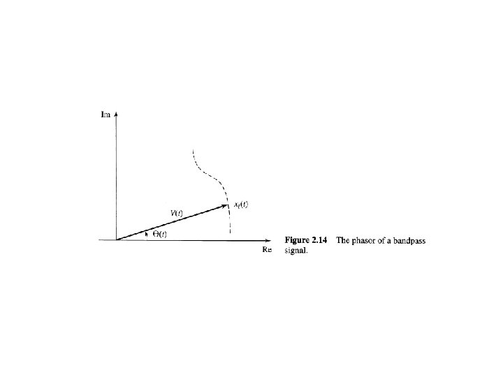
• Let be a monochromatic signal. Then it can also be represented as • The term is called the phasor corresponding to x(t). • The phasor contains the information about the amplitude and phase of the signal, but does not have any information concerning the frequency of it. • To find the output of a LTI circuit driven by this sinusoidal signal, it is enough to multiply the phase of the excitation signal by the value of the frequency response of the system computed at the input frequency to obtain the phasor corresponding to the output.

• Let be a monochromatic signal. Then it can also be represented as • The term is called the phasor corresponding to x(t). • The phasor contains the information about the amplitude and phase of the signal, but does not have any information concerning the frequency.

• But, the complex-valued signal contains the complete information about x(t) • Phasor X can be obtained from

• Note that the frequency domain representation of Z(f) is obtained by deleting the negative frequencies from X(f) and multiplying the positive frequencies by 2. By doing this, we have • From Table 2. 1, we have Duality Theorem

• For any bandpass signal x(t), we define its corresponding analytic signal by where • Comparing the above result with the case that x(t) is sinusoidal), we have • We see that plays the same role as • is called the Hilbert transform of

• By doing some frequency analysis on , we have • Hilbert transform is equivalent to a phase shift for positive frequency and phase shift for the negative frequency.

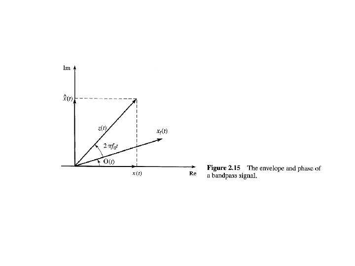
• The lowpass representation of the bandpass signal x(t) can be represented by and • is a lowpass signal which is in general a complex signal, i. e. , in-phase component quadrature component

• Substituting for and rewriting , we obtain • Equating the real and imaginary parts, we have

• Define the envelope and phase of x(t) as envelope phase We can write • Comparing to phasor relation , we can find that the only difference is that the envelope and phase are both time-varying functions.

• The function z(t) can also be expressed as • From above equations, we have

Bandpass Signal Lowpass Signal Analytic Signal

2. 5. 1 Transmission of Bandpass Signals through Bandpass Systems • Let x(t) be a bandpass signal with carrier frequency , and let h(t) be the impulse response of an LTI system. Let y(t) be the output of the system when driven by x(t). • In frequency domain we have Y(f)=X(f)H(f). The signal y(t) is also a bandpass signal.

• By writing H(f) and X(f) in terms of their lowpass equivalents, we obtain Multiplying these two relations, we have Finally, we obtain the frequency-domain relationship or its equivalent time-domain relationship • To obtain y(t), we can carry out the convolution at low frequency to obtain , and then transform to higher frequencies using

Relationship Between the Bandpass Signal and Its Lowpass Representation