Signals and Systems Analysis NET 351 Instructor Dr

Signals and Systems Analysis NET 351 Instructor: Dr. Amer El-Khairy ﻋﺎﻣﺮ ﺍﻟﺨﻴﺮﻱ. ﺩ

Linear-time invariant systems Two most important attributes of systems are linearity and time-invariance. • Develop the fundamental input-output relationship for systems having these attributes. • show that the input-output relationship for LTI systems is described in terms of a convolution operation. • The importance of the convolution operation in LTI • Systems from the fact that knowledge of the response of an LTI system to the unit impulse input allows us to find its output to any input signals. • Specify the input-output relationships for LTI systems by differential and difference equations. Signals and systems analysis ﻋﺎﻣﺮ ﺍﻟﺨﻴﺮﻱ. ﺩ 2

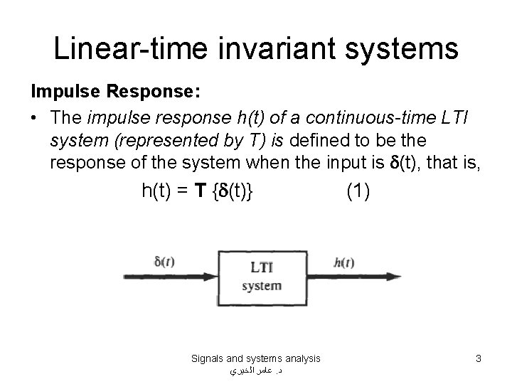
Linear-time invariant systems Impulse Response: • The impulse response h(t) of a continuous-time LTI system (represented by T) is defined to be the response of the system when the input is d(t), that is, h(t) = T {d(t)} Signals and systems analysis ﻋﺎﻣﺮ ﺍﻟﺨﻴﺮﻱ. ﺩ (1) 3

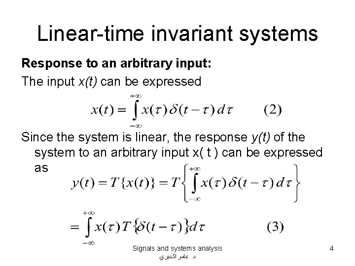
Linear-time invariant systems Response to an arbitrary input: The input x(t) can be expressed Since the system is linear, the response y(t) of the system to an arbitrary input x( t ) can be expressed as Signals and systems analysis ﻋﺎﻣﺮ ﺍﻟﺨﻴﺮﻱ. ﺩ 4

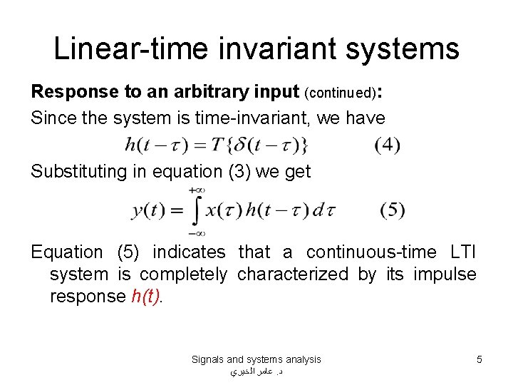
Linear-time invariant systems Response to an arbitrary input (continued): Since the system is time-invariant, we have Substituting in equation (3) we get Equation (5) indicates that a continuous-time LTI system is completely characterized by its impulse response h(t). Signals and systems analysis ﻋﺎﻣﺮ ﺍﻟﺨﻴﺮﻱ. ﺩ 5

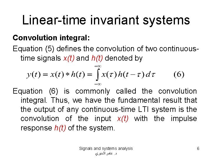
Linear-time invariant systems Convolution integral: Equation (5) defines the convolution of two continuoustime signals x(t) and h(t) denoted by Equation (6) is commonly called the convolution integral. Thus, we have the fundamental result that the output of any continuous-time LTI system is the convolution of the input x(t) with the impulse response h(t) of the system. Signals and systems analysis ﻋﺎﻣﺮ ﺍﻟﺨﻴﺮﻱ. ﺩ 6

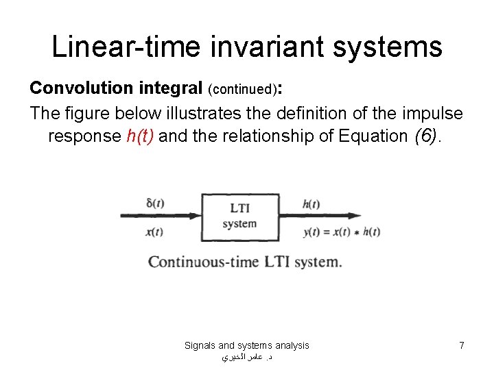
Linear-time invariant systems Convolution integral (continued): The figure below illustrates the definition of the impulse response h(t) and the relationship of Equation (6). Signals and systems analysis ﻋﺎﻣﺮ ﺍﻟﺨﻴﺮﻱ. ﺩ 7

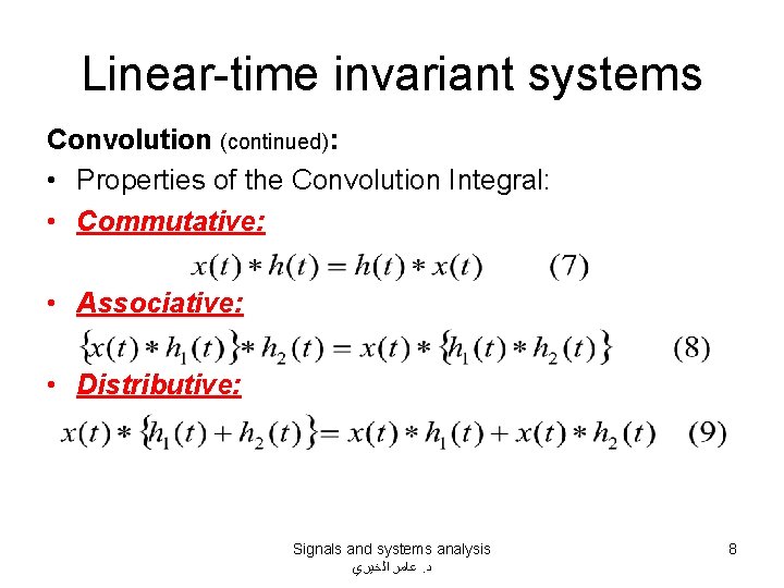
Linear-time invariant systems Convolution (continued): • Properties of the Convolution Integral: • Commutative: • Associative: • Distributive: Signals and systems analysis ﻋﺎﻣﺮ ﺍﻟﺨﻴﺮﻱ. ﺩ 8

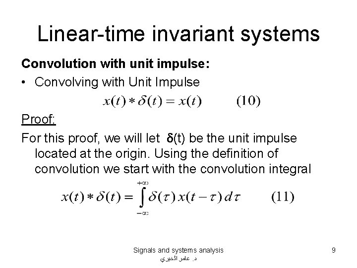
Linear-time invariant systems Convolution with unit impulse: • Convolving with Unit Impulse Proof: For this proof, we will let d(t) be the unit impulse located at the origin. Using the definition of convolution we start with the convolution integral Signals and systems analysis ﻋﺎﻣﺮ ﺍﻟﺨﻴﺮﻱ. ﺩ 9

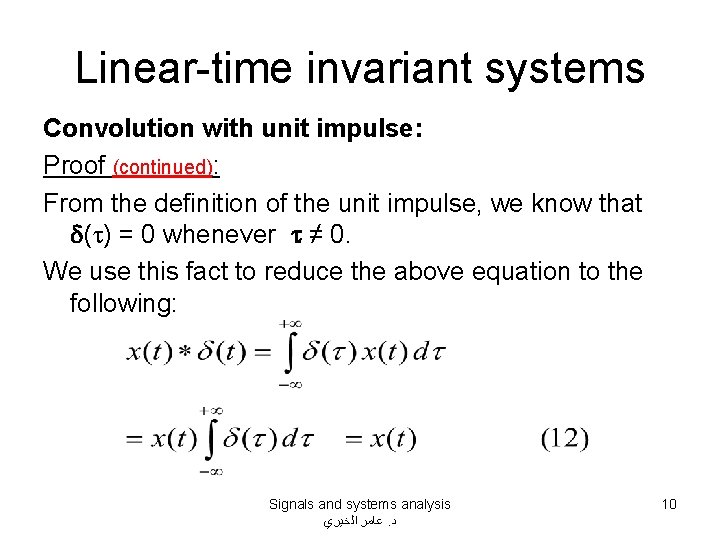
Linear-time invariant systems Convolution with unit impulse: Proof (continued): From the definition of the unit impulse, we know that d(t) = 0 whenever t ≠ 0. We use this fact to reduce the above equation to the following: Signals and systems analysis ﻋﺎﻣﺮ ﺍﻟﺨﻴﺮﻱ. ﺩ 10

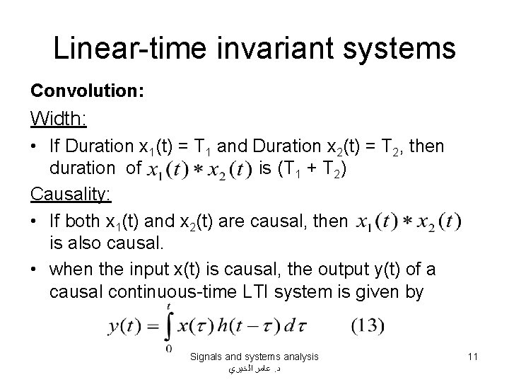
Linear-time invariant systems Convolution: Width: • If Duration x 1(t) = T 1 and Duration x 2(t) = T 2, then duration of is (T 1 + T 2) Causality: • If both x 1(t) and x 2(t) are causal, then is also causal. • when the input x(t) is causal, the output y(t) of a causal continuous-time LTI system is given by Signals and systems analysis ﻋﺎﻣﺮ ﺍﻟﺨﻴﺮﻱ. ﺩ 11

Discrete LTI systems Impulse Response: The impulse response (or unit sample response) h[n] of a discrete-time LTI system (represented by T) is defined to be the response of the system when the input is d[n], that is, Response to an Arbitrary Input: As we know, an input x[n] can be expressed as Signals and systems analysis ﻋﺎﻣﺮ ﺍﻟﺨﻴﺮﻱ. ﺩ 12

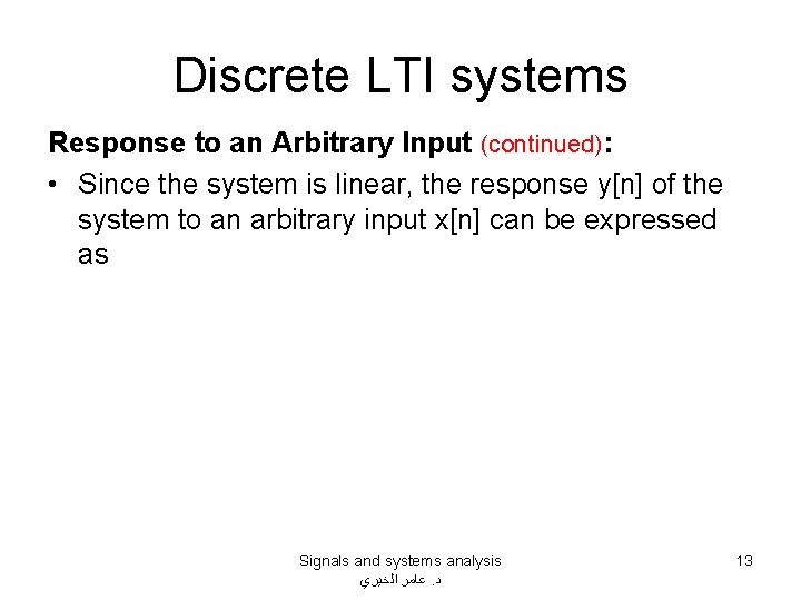
Discrete LTI systems Response to an Arbitrary Input (continued): • Since the system is linear, the response y[n] of the system to an arbitrary input x[n] can be expressed as Signals and systems analysis ﻋﺎﻣﺮ ﺍﻟﺨﻴﺮﻱ. ﺩ 13

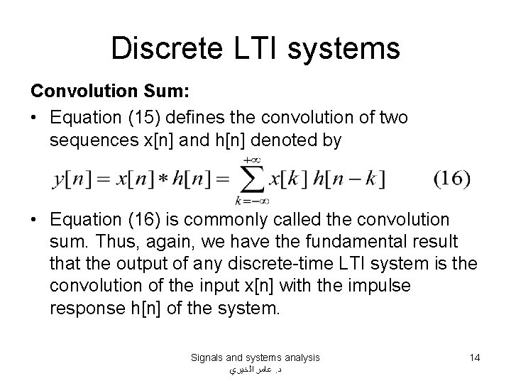
Discrete LTI systems Convolution Sum: • Equation (15) defines the convolution of two sequences x[n] and h[n] denoted by • Equation (16) is commonly called the convolution sum. Thus, again, we have the fundamental result that the output of any discrete-time LTI system is the convolution of the input x[n] with the impulse response h[n] of the system. Signals and systems analysis ﻋﺎﻣﺮ ﺍﻟﺨﻴﺮﻱ. ﺩ 14

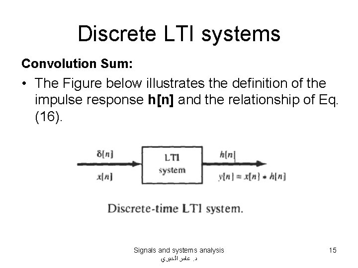
Discrete LTI systems Convolution Sum: • The Figure below illustrates the definition of the impulse response h[n] and the relationship of Eq. (16). Signals and systems analysis ﻋﺎﻣﺮ ﺍﻟﺨﻴﺮﻱ. ﺩ 15

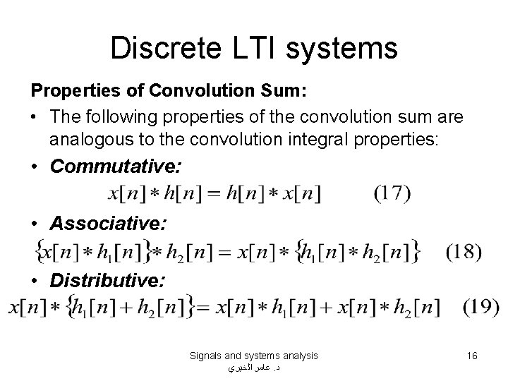
Discrete LTI systems Properties of Convolution Sum: • The following properties of the convolution sum are analogous to the convolution integral properties: • Commutative: • Associative: • Distributive: Signals and systems analysis ﻋﺎﻣﺮ ﺍﻟﺨﻴﺮﻱ. ﺩ 16

Discrete LTI systems • Step Response: The step response s[n] of a discrete-time LTI system with the impulse response h[n] is readily obtained from Eq. (20) Signals and systems analysis ﻋﺎﻣﺮ ﺍﻟﺨﻴﺮﻱ. ﺩ 17

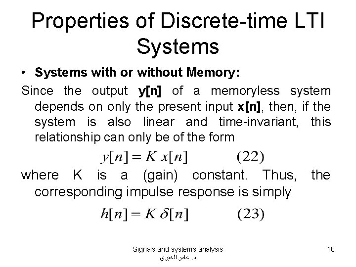
Properties of Discrete-time LTI Systems • Systems with or without Memory: Since the output y[n] of a memoryless system depends on only the present input x[n], then, if the system is also linear and time-invariant, this relationship can only be of the form where K is a (gain) constant. Thus, corresponding impulse response is simply Signals and systems analysis ﻋﺎﻣﺮ ﺍﻟﺨﻴﺮﻱ. ﺩ the 18

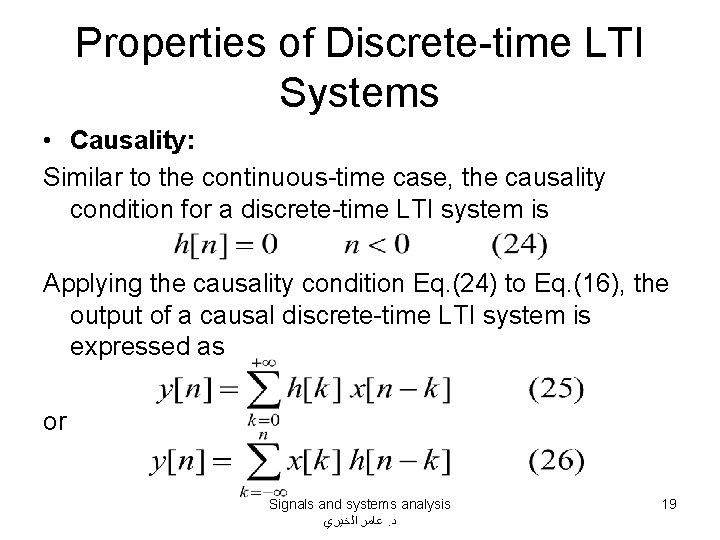
Properties of Discrete-time LTI Systems • Causality: Similar to the continuous-time case, the causality condition for a discrete-time LTI system is Applying the causality condition Eq. (24) to Eq. (16), the output of a causal discrete-time LTI system is expressed as or Signals and systems analysis ﻋﺎﻣﺮ ﺍﻟﺨﻴﺮﻱ. ﺩ 19

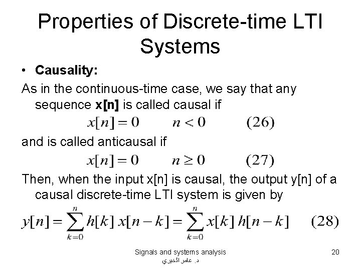
Properties of Discrete-time LTI Systems • Causality: As in the continuous-time case, we say that any sequence x[n] is called causal if and is called anticausal if Then, when the input x[n] is causal, the output y[n] of a causal discrete-time LTI system is given by Signals and systems analysis ﻋﺎﻣﺮ ﺍﻟﺨﻴﺮﻱ. ﺩ 20

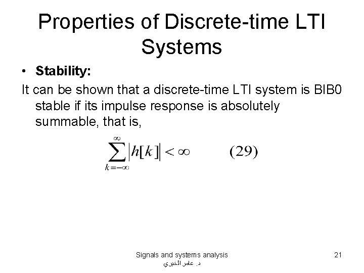
Properties of Discrete-time LTI Systems • Stability: It can be shown that a discrete-time LTI system is BIB 0 stable if its impulse response is absolutely summable, that is, Signals and systems analysis ﻋﺎﻣﺮ ﺍﻟﺨﻴﺮﻱ. ﺩ 21

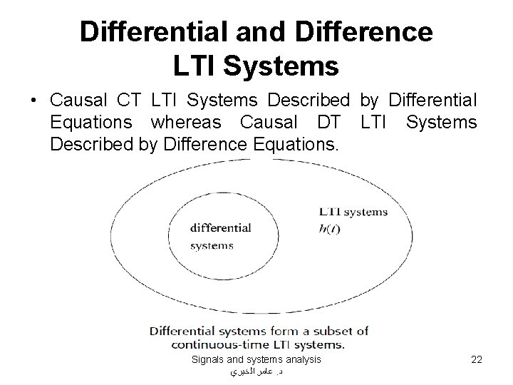
Differential and Difference LTI Systems • Causal CT LTI Systems Described by Differential Equations whereas Causal DT LTI Systems Described by Difference Equations. Signals and systems analysis ﻋﺎﻣﺮ ﺍﻟﺨﻴﺮﻱ. ﺩ 22

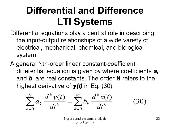
Differential and Difference LTI Systems Differential equations play a central role in describing the input-output relationships of a wide variety of electrical, mechanical, chemical, and biological system A general Nth-order linear constant-coefficient differential equation is given by where coefficients a, and b, are real constants. The order N refers to the highest derivative of y(t) in Eq. (30). Signals and systems analysis ﻋﺎﻣﺮ ﺍﻟﺨﻴﺮﻱ. ﺩ 23

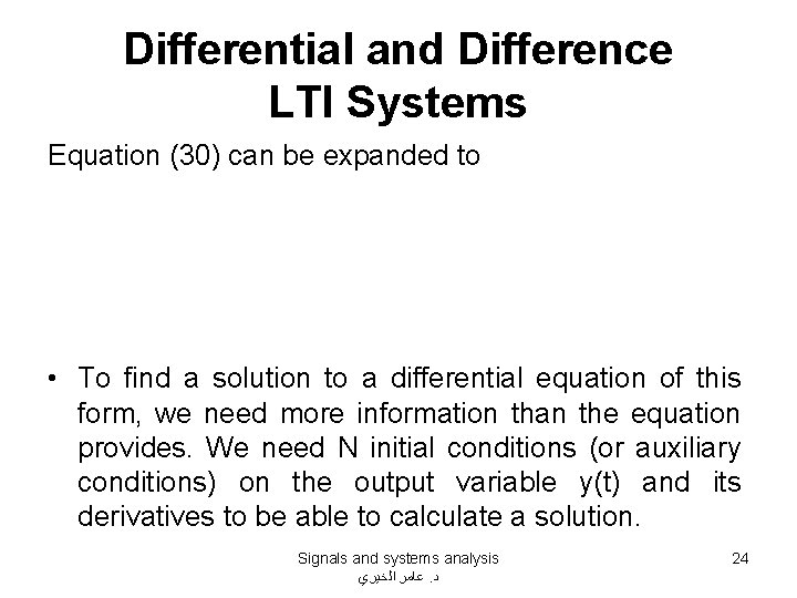
Differential and Difference LTI Systems Equation (30) can be expanded to • To find a solution to a differential equation of this form, we need more information than the equation provides. We need N initial conditions (or auxiliary conditions) on the output variable y(t) and its derivatives to be able to calculate a solution. Signals and systems analysis ﻋﺎﻣﺮ ﺍﻟﺨﻴﺮﻱ. ﺩ 24

Differential and Difference LTI Systems The complete solution to Eq. (30) is given by the sum of the homogeneous solution of the differential equation (a solution with the input signal set to zero) and of a particular solution (an output signal that satisfies the differential equation), also called the forced response of the system. The usual terminology is as follows: • Forced response of the system = particular solution (usually has the same form as the input signal). • Natural response of the system = homogeneous solution (depends on initial conditions and forced Signals and systems analysis 25 response) ﻋﺎﻣﺮ ﺍﻟﺨﻴﺮﻱ. ﺩ

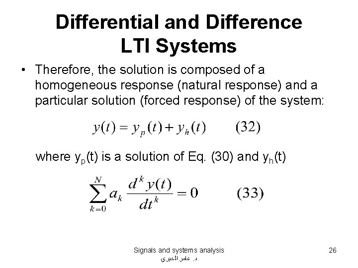
Differential and Difference LTI Systems • Therefore, the solution is composed of a homogeneous response (natural response) and a particular solution (forced response) of the system: where yp(t) is a solution of Eq. (30) and yh(t) Signals and systems analysis ﻋﺎﻣﺮ ﺍﻟﺨﻴﺮﻱ. ﺩ 26

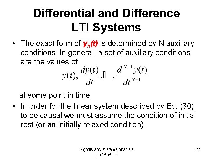
Differential and Difference LTI Systems • The exact form of yh(t) is determined by N auxiliary conditions. In general, a set of auxiliary conditions are the values of at some point in time. • In order for the linear system described by Eq. (30) to be causal we must assume the condition of initial rest (or an initially relaxed condition). Signals and systems analysis ﻋﺎﻣﺮ ﺍﻟﺨﻴﺮﻱ. ﺩ 27

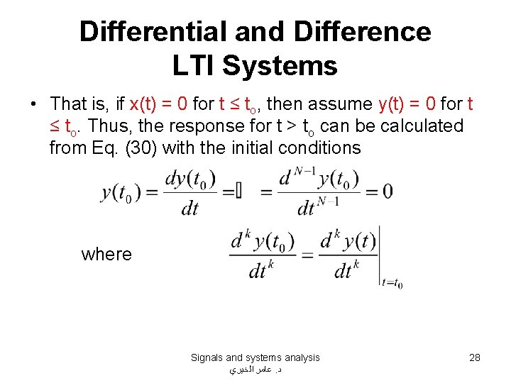
Differential and Difference LTI Systems • That is, if x(t) = 0 for t ≤ to, then assume y(t) = 0 for t ≤ to. Thus, the response for t > to can be calculated from Eq. (30) with the initial conditions where Signals and systems analysis ﻋﺎﻣﺮ ﺍﻟﺨﻴﺮﻱ. ﺩ 28

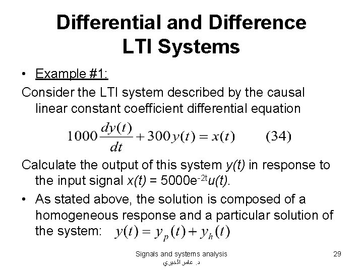
Differential and Difference LTI Systems • Example #1: Consider the LTI system described by the causal linear constant coefficient differential equation Calculate the output of this system y(t) in response to the input signal x(t) = 5000 e-2 tu(t). • As stated above, the solution is composed of a homogeneous response and a particular solution of the system: Signals and systems analysis ﻋﺎﻣﺮ ﺍﻟﺨﻴﺮﻱ. ﺩ 29

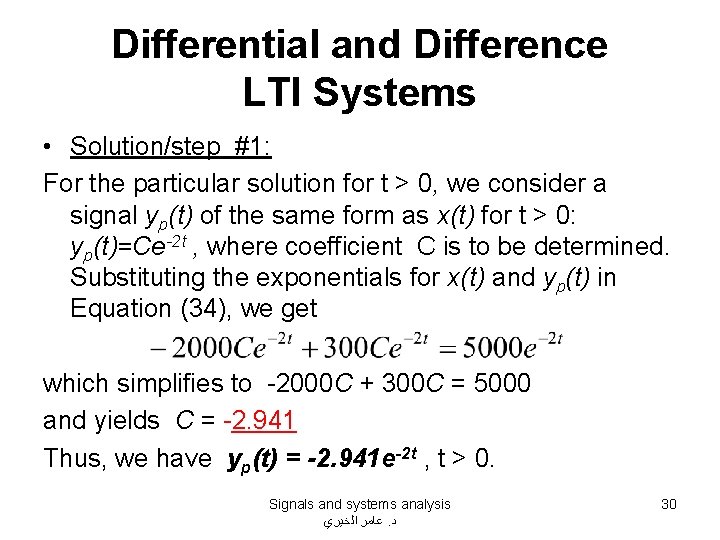
Differential and Difference LTI Systems • Solution/step #1: For the particular solution for t > 0, we consider a signal yp(t) of the same form as x(t) for t > 0: yp(t)=Ce-2 t , where coefficient C is to be determined. Substituting the exponentials for x(t) and yp(t) in Equation (34), we get which simplifies to -2000 C + 300 C = 5000 and yields C = -2. 941 Thus, we have yp(t) = -2. 941 e-2 t , t > 0. Signals and systems analysis ﻋﺎﻣﺮ ﺍﻟﺨﻴﺮﻱ. ﺩ 30

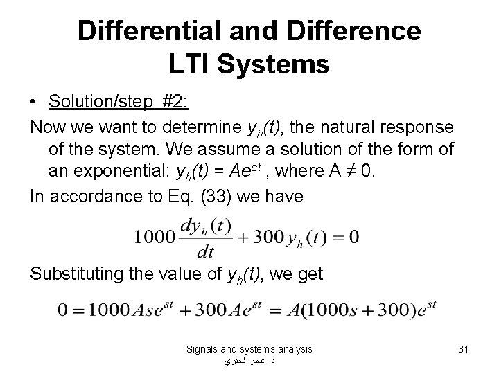
Differential and Difference LTI Systems • Solution/step #2: Now we want to determine yh(t), the natural response of the system. We assume a solution of the form of an exponential: yh(t) = Aest , where A ≠ 0. In accordance to Eq. (33) we have Substituting the value of yh(t), we get Signals and systems analysis ﻋﺎﻣﺮ ﺍﻟﺨﻴﺮﻱ. ﺩ 31

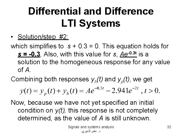
Differential and Difference LTI Systems • Solution/step #2: which simplifies to s + 0. 3 = 0. This equation holds for s = -0. 3. Also, with this value for s, Ae-0. 3 t is a solution to the homogeneous response for any value of A. Combining both responses yh(t) and yp(t), we get Now, because we have not yet specified an initial condition on y(t), this response is not completely determined, as the value of A is still unknown. Signals and systems analysis ﻋﺎﻣﺮ ﺍﻟﺨﻴﺮﻱ. ﺩ 32

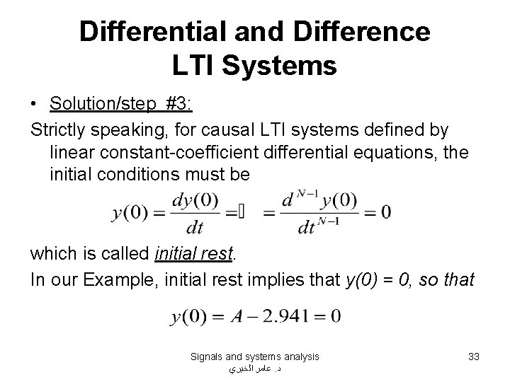
Differential and Difference LTI Systems • Solution/step #3: Strictly speaking, for causal LTI systems defined by linear constant-coefficient differential equations, the initial conditions must be which is called initial rest. In our Example, initial rest implies that y(0) = 0, so that Signals and systems analysis ﻋﺎﻣﺮ ﺍﻟﺨﻴﺮﻱ. ﺩ 33

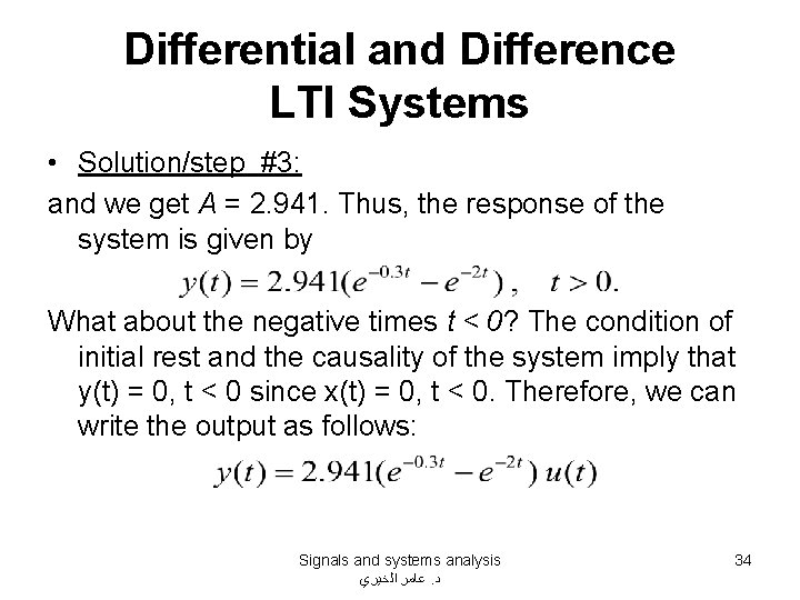
Differential and Difference LTI Systems • Solution/step #3: and we get A = 2. 941. Thus, the response of the system is given by What about the negative times t < 0? The condition of initial rest and the causality of the system imply that y(t) = 0, t < 0 since x(t) = 0, t < 0. Therefore, we can write the output as follows: Signals and systems analysis ﻋﺎﻣﺮ ﺍﻟﺨﻴﺮﻱ. ﺩ 34

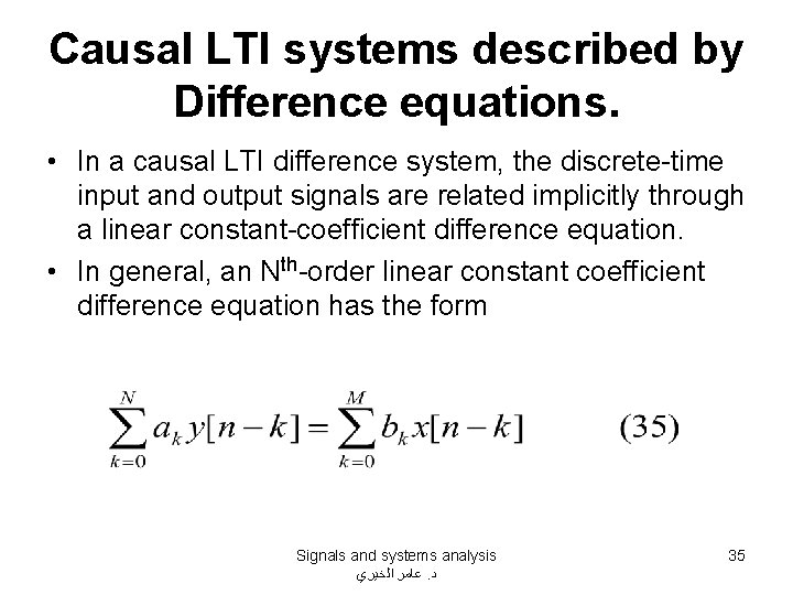
Causal LTI systems described by Difference equations. • In a causal LTI difference system, the discrete-time input and output signals are related implicitly through a linear constant-coefficient difference equation. • In general, an Nth-order linear constant coefficient difference equation has the form Signals and systems analysis ﻋﺎﻣﺮ ﺍﻟﺨﻴﺮﻱ. ﺩ 35

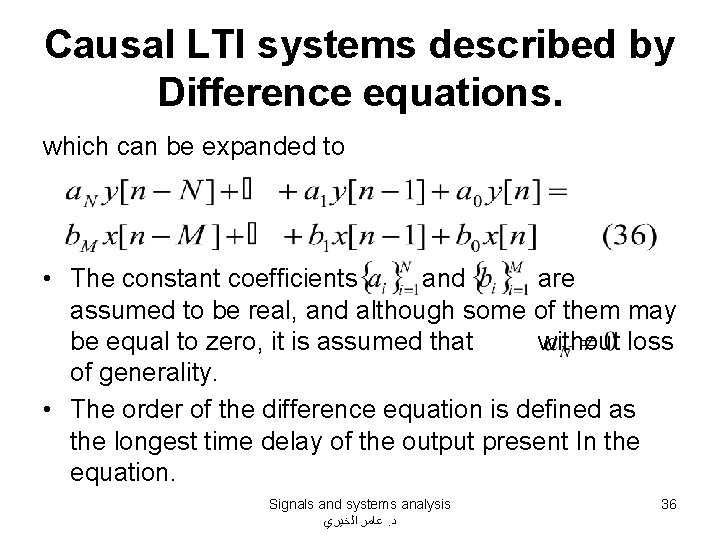
Causal LTI systems described by Difference equations. which can be expanded to • The constant coefficients and are assumed to be real, and although some of them may be equal to zero, it is assumed that without loss of generality. • The order of the difference equation is defined as the longest time delay of the output present In the equation. Signals and systems analysis ﻋﺎﻣﺮ ﺍﻟﺨﻴﺮﻱ. ﺩ 36

Causal LTI systems described by Difference equations. • To find a solution to the difference equation, we need more information than what the equation provides. We need N initial conditions (or auxiliary conditions) on the output variable (its N past values) to be able to compute a specific solution. Signals and systems analysis ﻋﺎﻣﺮ ﺍﻟﺨﻴﺮﻱ. ﺩ 37

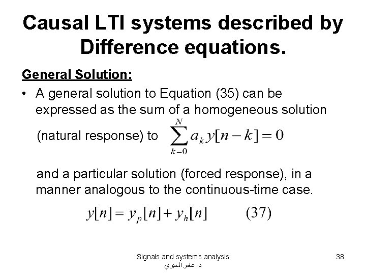
Causal LTI systems described by Difference equations. General Solution: • A general solution to Equation (35) can be expressed as the sum of a homogeneous solution (natural response) to and a particular solution (forced response), in a manner analogous to the continuous-time case. Signals and systems analysis ﻋﺎﻣﺮ ﺍﻟﺨﻴﺮﻱ. ﺩ 38

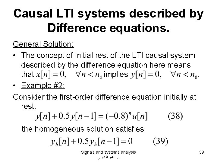
Causal LTI systems described by Difference equations. General Solution: • The concept of initial rest of the LTI causal system described by the difference equation here means that implies. • Example #2: Consider the first-order difference equation initially at rest: the homogeneous solution satisfies Signals and systems analysis ﻋﺎﻣﺮ ﺍﻟﺨﻴﺮﻱ. ﺩ 39

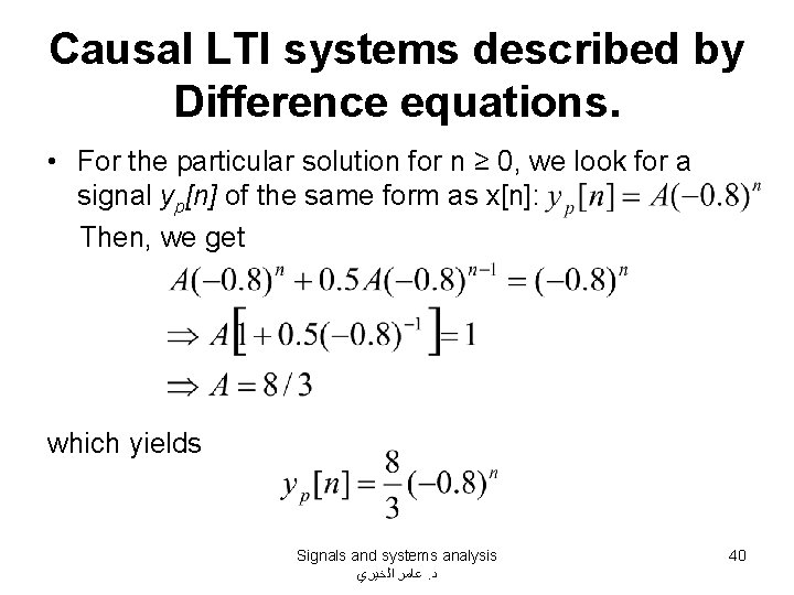
Causal LTI systems described by Difference equations. • For the particular solution for n ≥ 0, we look for a signal yp[n] of the same form as x[n]: Then, we get which yields Signals and systems analysis ﻋﺎﻣﺮ ﺍﻟﺨﻴﺮﻱ. ﺩ 40

Causal LTI systems described by Difference equations. • Now let us determine yh[n], the natural response of the system. We hypothesize a solution of the form of an exponential signal: . Substituting this exponential in Equation (39), we get • With this value for z, is a solution to the homogeneous equation for any choice of B. Signals and systems analysis ﻋﺎﻣﺮ ﺍﻟﺨﻴﺮﻱ. ﺩ 41

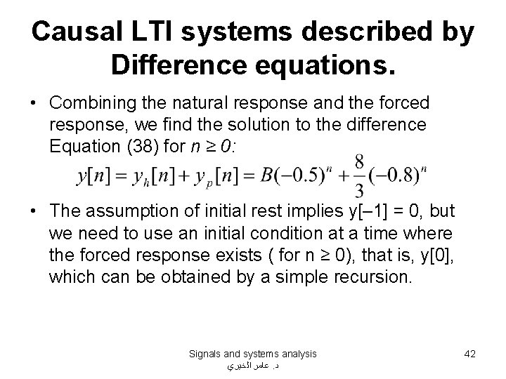
Causal LTI systems described by Difference equations. • Combining the natural response and the forced response, we find the solution to the difference Equation (38) for n ≥ 0: • The assumption of initial rest implies y[– 1] = 0, but we need to use an initial condition at a time where the forced response exists ( for n ≥ 0), that is, y[0], which can be obtained by a simple recursion. Signals and systems analysis ﻋﺎﻣﺮ ﺍﻟﺨﻴﺮﻱ. ﺩ 42

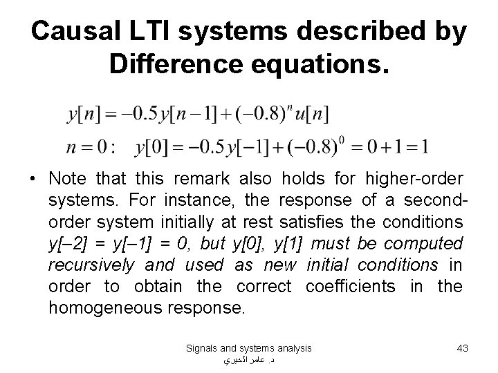
Causal LTI systems described by Difference equations. • Note that this remark also holds for higher-order systems. For instance, the response of a secondorder system initially at rest satisfies the conditions y[– 2] = y[– 1] = 0, but y[0], y[1] must be computed recursively and used as new initial conditions in order to obtain the correct coefficients in the homogeneous response. Signals and systems analysis ﻋﺎﻣﺮ ﺍﻟﺨﻴﺮﻱ. ﺩ 43

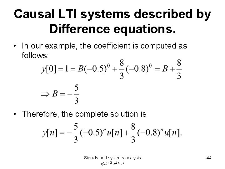
Causal LTI systems described by Difference equations. • In our example, the coefficient is computed as follows: • Therefore, the complete solution is Signals and systems analysis ﻋﺎﻣﺮ ﺍﻟﺨﻴﺮﻱ. ﺩ 44