DiscreteTime signals and systems 1 Introduction l Signal

Discrete-Time signals and systems 1

Introduction l Signal: A signal can be defined as a function that conveys information, generally about the state or behavior of a physical system. l Continuous-time signal: Continuous-time signals are defined along a continuum of times and thus are represented by a continuous independent variable. Continuous-time signals are often referred to as analog signals. l Discrete time signal: Discrete-time signals are defined at discrete times and thus the independent variable has discrete values; i. e. , discrete-time signals are represented as sequences of number. 2

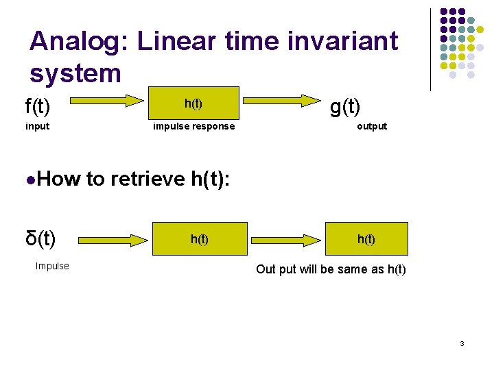
Analog: Linear time invariant system f(t) h(t) input impulse response l. How δ(t) Impulse g(t) output to retrieve h(t): h(t) Out put will be same as h(t) 3

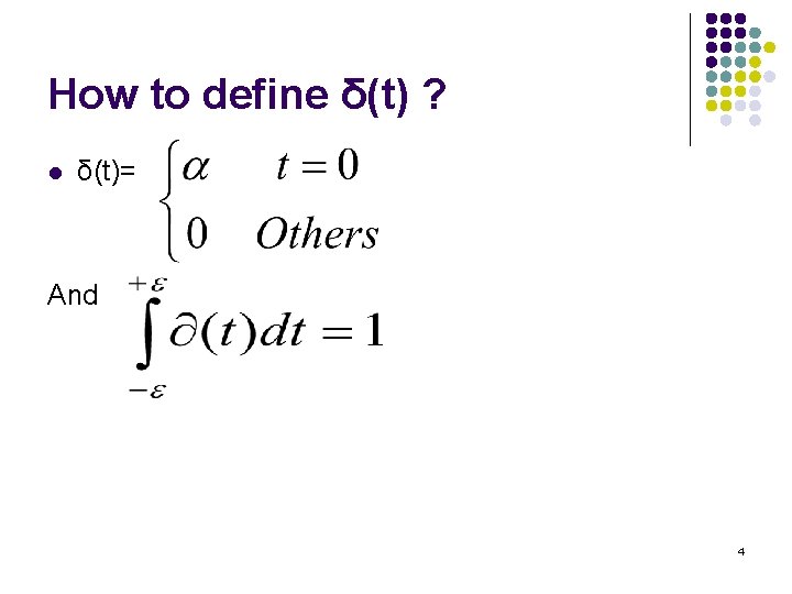
How to define δ(t) ? l δ(t)= And 4

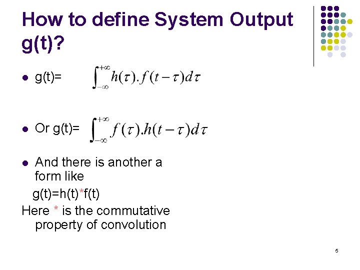
How to define System Output g(t)? l g(t)= l Or g(t)= And there is another a form like g(t)=h(t)*f(t) Here * is the commutative property of convolution l 5

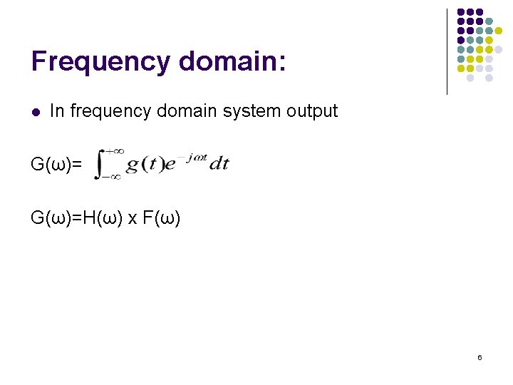
Frequency domain: l In frequency domain system output G(ω)=H(ω) x F(ω) 6

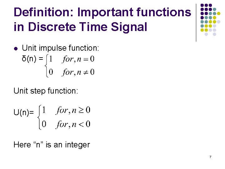
Definition: Important functions in Discrete Time Signal l Unit impulse function: δ(n) = Unit step function: U(n)= Here “n” is an integer 7

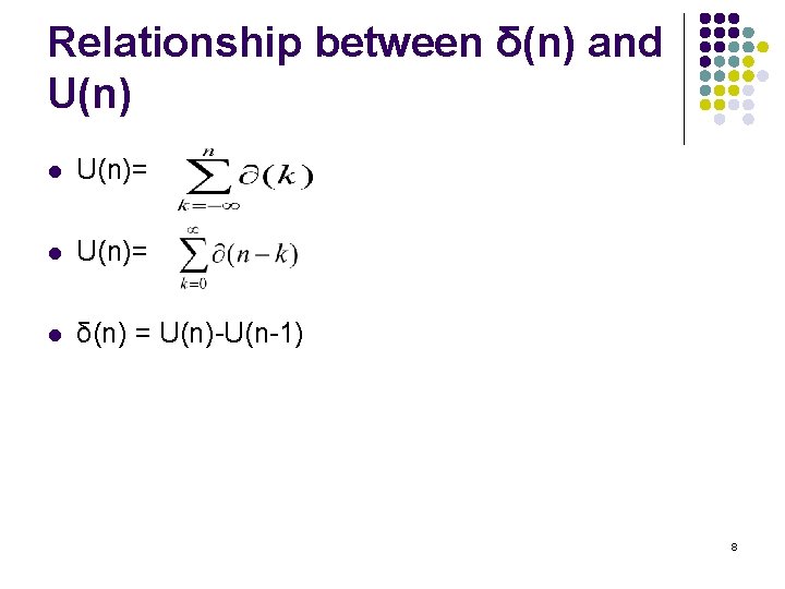
Relationship between δ(n) and U(n) l U(n)= l δ(n) = U(n)-U(n-1) 8

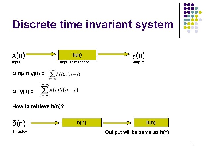
Discrete time invariant system x(n) input h(n) impulse response y(n) output Output y(n) = Or y(n) = How to retrieve h(n)? δ(n) Impulse h(n) Out put will be same as h(n) 9

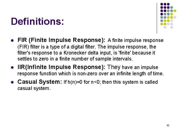
Definitions: l FIR (Finite Impulse Response): A finite impulse response (FIR) filter is a type of a digital filter. The impulse response, the filter's response to a Kronecker delta input, is 'finite' because it settles to zero in a finite number of sample intervals. l IIR(Infinite Impulse Response): They have an impulse response function which is non-zero over an infinite length of time. l Casual System: If h(n)=0 for n<0; then this system is called casual system. 10

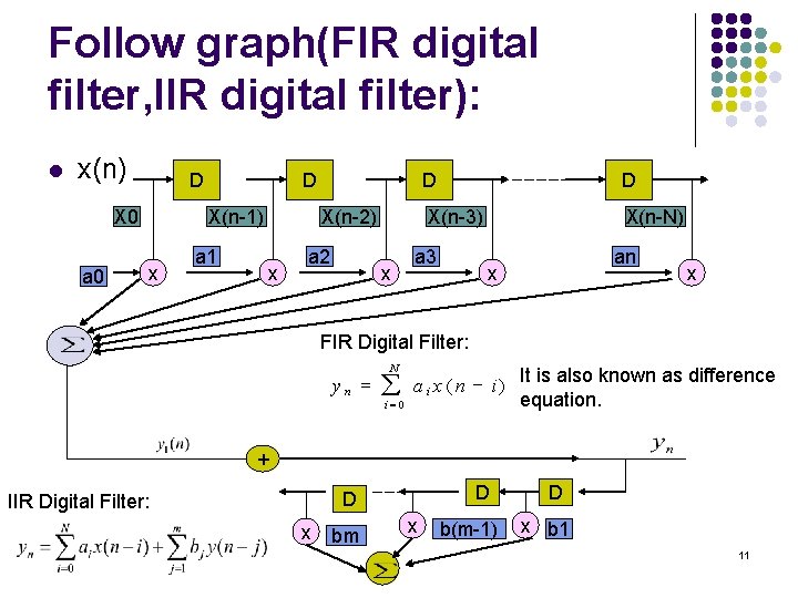
Follow graph(FIR digital filter, IIR digital filter): l x(n) D X 0 a 0 D X(n-1) x a 1 D X(n-2) x a 2 D X(n-3) x a 3 X(n-N) an x x FIR Digital Filter: yn = N å i=0 a i x ( n - i ) It is also known as difference equation. + D D IIR Digital Filter: x bm x b(m-1) D x b 1 11

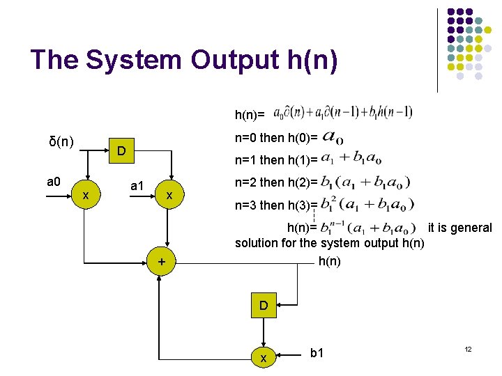
The System Output h(n)= δ(n) a 0 n=0 then h(0)= D x n=1 then h(1)= a 1 x + n=2 then h(2)= n=3 then h(3)= h(n)= it is general solution for the system output h(n) D x b 1 12

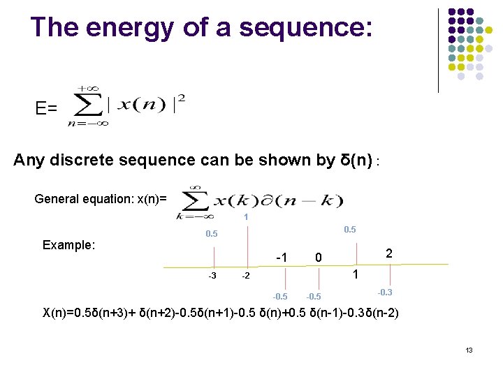
The energy of a sequence: E= Any discrete sequence can be shown by δ(n) : General equation: x(n)= 1 Example: 0. 5 -1 -3 2 0 1 -2 -0. 5 -0. 3 X(n)=0. 5δ(n+3)+ δ(n+2)-0. 5δ(n+1)-0. 5 δ(n)+0. 5 δ(n-1)-0. 3δ(n-2) 13

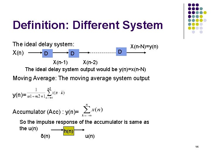
Definition: Different System The ideal delay system: X(n) D D D X(n-N)=y(n) X(n-1) X(n-2) The ideal delay system output would be y(n)=x(n-N) Moving Average: The moving average system output y(n)= Accumulator (Acc) : y(n)= So the impulse response of the accumulator is same as the u(n) h(n) δ(n) u(n) 14

Linear Shift Invariant System a 1 x 1(n) x + X 2(n) [ T[. ] ] x a 1 a 2 x 1(n) T [. ] X 2(n) T [. ] y 1(n) y 2(n) x + x If a 2 y’ = y’’ then system is linear 15

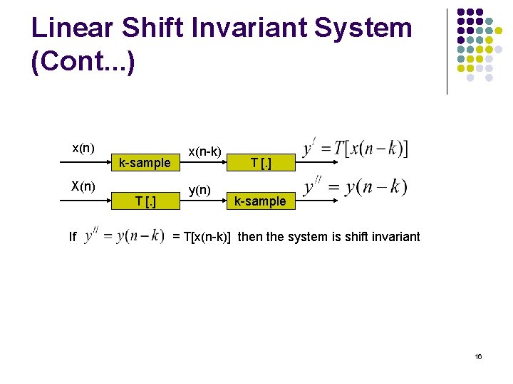
Linear Shift Invariant System (Cont. . . ) x(n) k-sample X(n) T [. ] If x(n-k) y(n) T [. ] k-sample = T[x(n-k)] then the system is shift invariant 16

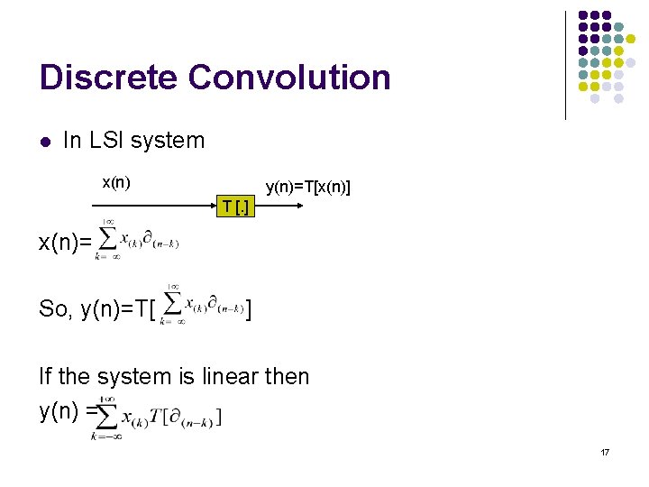
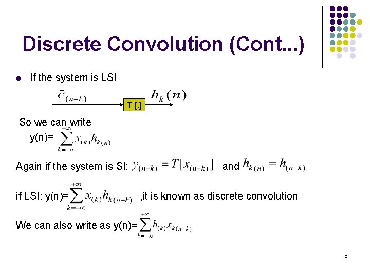
Discrete Convolution l In LSI system x(n) y(n)=T[x(n)] T [. ] x(n)= So, y(n)=T[ ] If the system is linear then y(n) = 17

Discrete Convolution (Cont. . . ) l If the system is LSI T [. ] So we can write y(n)= Again if the system is SI: if LSI: y(n)= and , it is known as discrete convolution We can also write as y(n)= 18

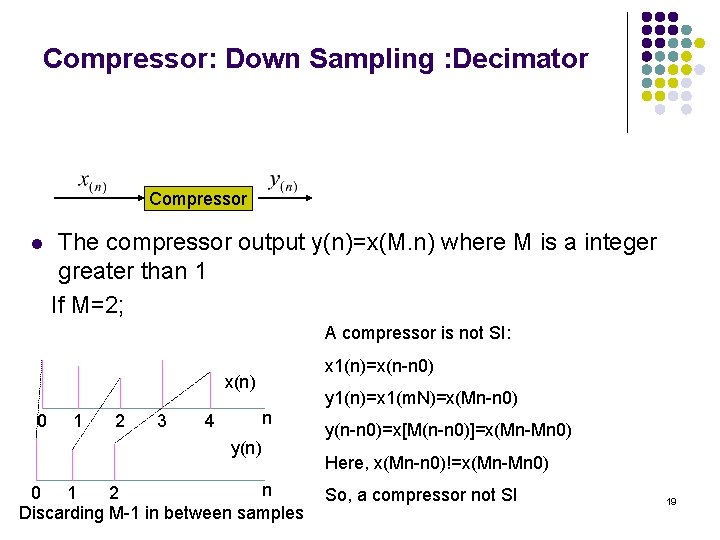
Compressor: Down Sampling : Decimator Compressor l The compressor output y(n)=x(M. n) where M is a integer greater than 1 If M=2; A compressor is not SI: x 1(n)=x(n-n 0) x(n) 0 1 2 3 n 4 y(n) n 0 1 2 Discarding M-1 in between samples y 1(n)=x 1(m. N)=x(Mn-n 0) y(n-n 0)=x[M(n-n 0)]=x(Mn-Mn 0) Here, x(Mn-n 0)!=x(Mn-Mn 0) So, a compressor not SI 19

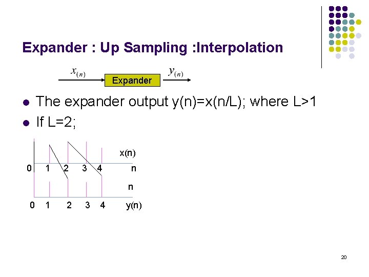
Expander : Up Sampling : Interpolation Expander l l The expander output y(n)=x(n/L); where L>1 If L=2; x(n) 0 1 2 3 4 n n 0 1 2 3 4 y(n) 20

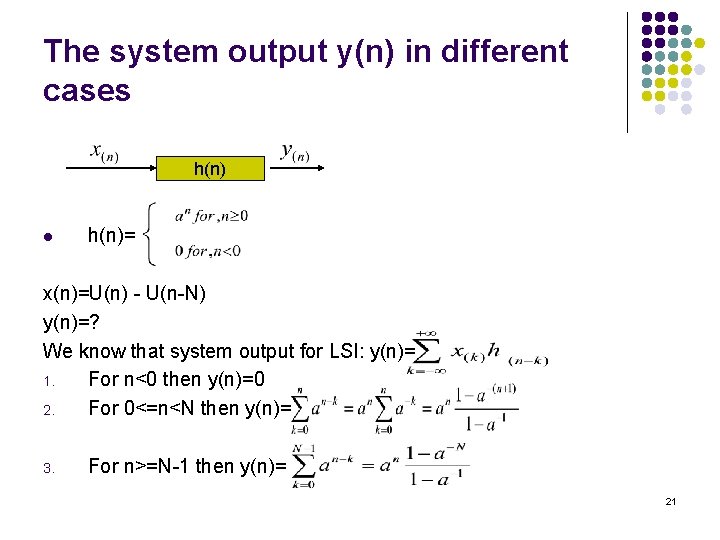
The system output y(n) in different cases h(n) l h(n)= x(n)=U(n) - U(n-N) y(n)=? We know that system output for LSI: y(n)= 1. For n<0 then y(n)=0 2. For 0<=n<N then y(n)= 3. For n>=N-1 then y(n)= 21

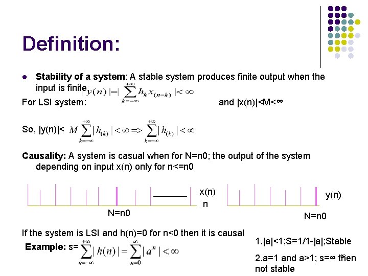
Definition: l Stability of a system: A stable system produces finite output when the input is finite. and |x(n)|<M< ∞ For LSI system: So, |y(n)|< Causality: A system is casual when for N=n 0; the output of the system depending on input x(n) only for n<=n 0 N=n 0 x(n) n If the system is LSI and h(n)=0 for n<0 then it is causal Example: s= y(n) N=n 0 1. |a|<1; S=1/1 -|a|; Stable 22 2. a=1 and a>1; s=∞ then not stable

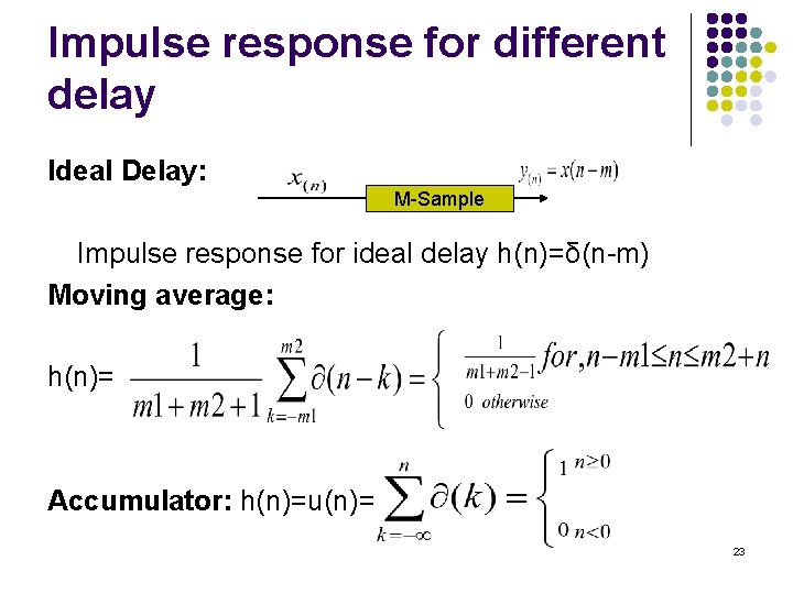
Impulse response for different delay Ideal Delay: M-Sample Impulse response for ideal delay h(n)=δ(n-m) Moving average: h(n)= Accumulator: h(n)=u(n)= 23

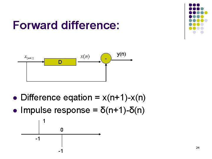
Forward difference: D l l - y(n) Difference eqation = x(n+1)-x(n) Impulse response = δ(n+1)-δ(n) 1 0 -1 -1 24

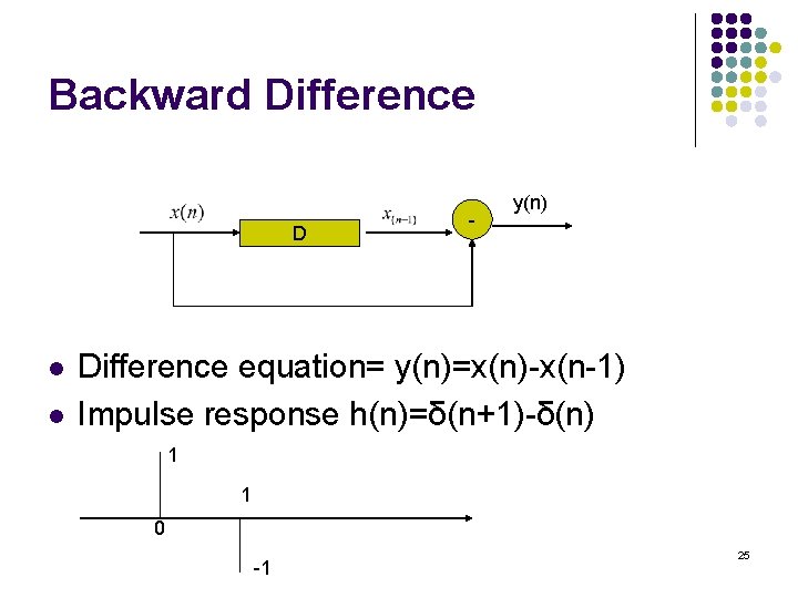
Backward Difference D l l - y(n) Difference equation= y(n)=x(n)-x(n-1) Impulse response h(n)=δ(n+1)-δ(n) 1 1 0 -1 25

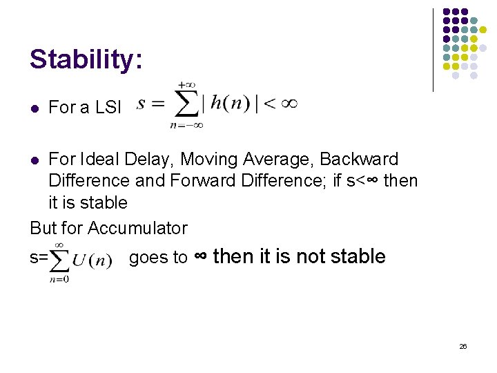
Stability: l For a LSI For Ideal Delay, Moving Average, Backward Difference and Forward Difference; if s<∞ then it is stable But for Accumulator l s= goes to ∞ then it is not stable 26

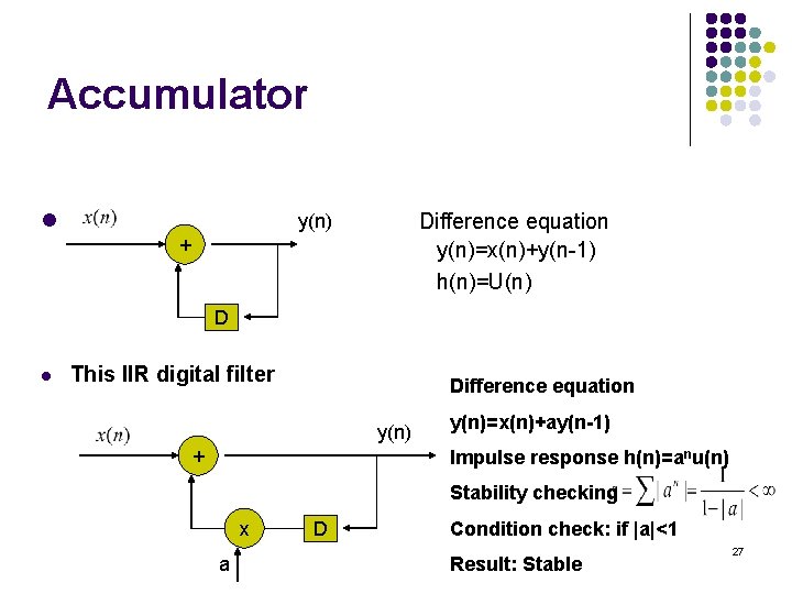
Accumulator l Difference equation y(n)=x(n)+y(n-1) h(n)=U(n) y(n) + D l This IIR digital filter Difference equation y(n) + y(n)=x(n)+ay(n-1) Impulse response h(n)=anu(n) Stability checking x a D Condition check: if |a|<1 Result: Stable 27

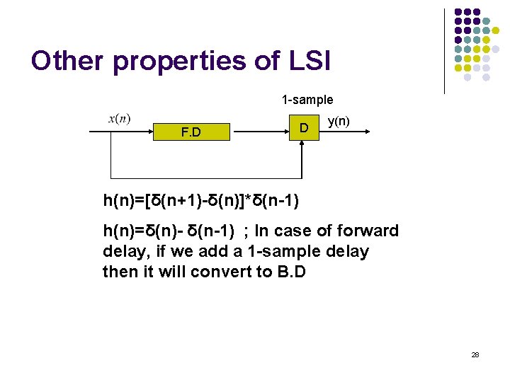
Other properties of LSI 1 -sample F. D D y(n) h(n)=[δ(n+1)-δ(n)]*δ(n-1) h(n)=δ(n)- δ(n-1) ; In case of forward delay, if we add a 1 -sample delay then it will convert to B. D 28

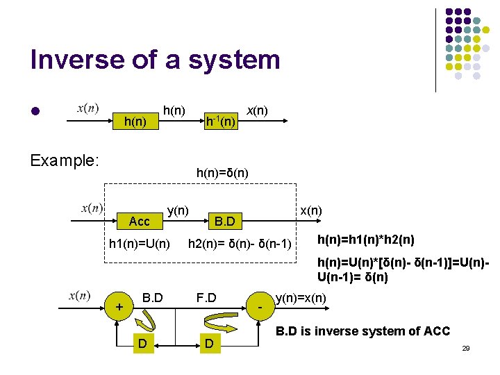
Inverse of a system l h(n) h-1(n) Example: x(n) h(n)=δ(n) Acc y(n) h 1(n)=U(n) x(n) B. D h 2(n)= δ(n)- δ(n-1) h(n)=h 1(n)*h 2(n) h(n)=U(n)*[δ(n)- δ(n-1)]=U(n)U(n-1)= δ(n) + B. D D F. D D - y(n)=x(n) B. D is inverse system of ACC 29

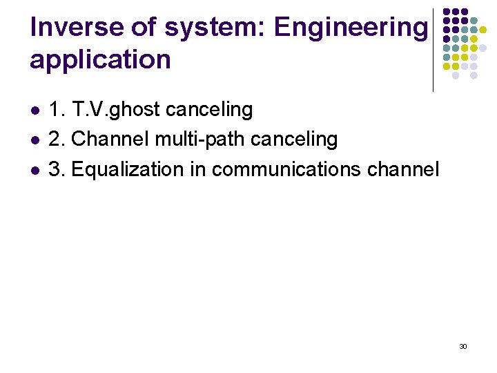
Inverse of system: Engineering application l l l 1. T. V. ghost canceling 2. Channel multi-path canceling 3. Equalization in communications channel 30

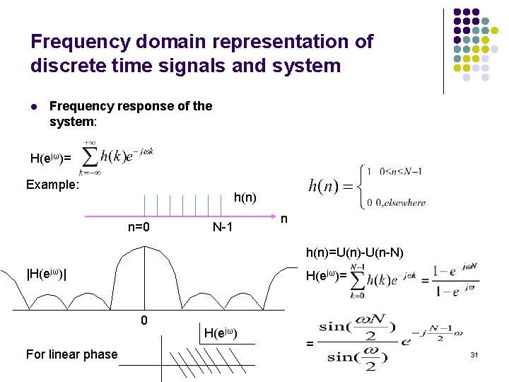
Frequency domain representation of discrete time signals and system l Frequency response of the system: H(ejω)= Example: h(n) n=0 N-1 n h(n)=U(n)-U(n-N) |H(ejω)| H(ejω)= 0 For linear phase H(ejω) = 31

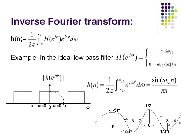
Inverse Fourier transform: h(n)= Example: In the ideal low pass filter -π -ωc 0 0 ωc 0 π ω 1/2 -1/5π -4 -3 -2 -5 -1/3π 2 -1 0 1 3 32 1/3π 4

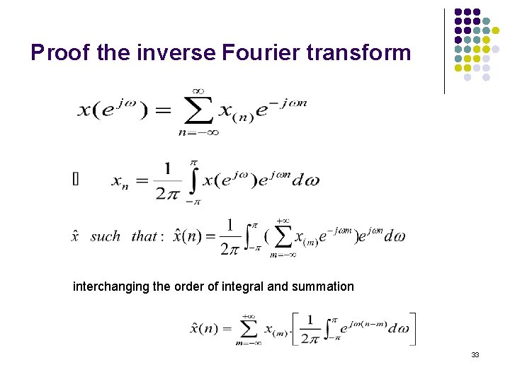
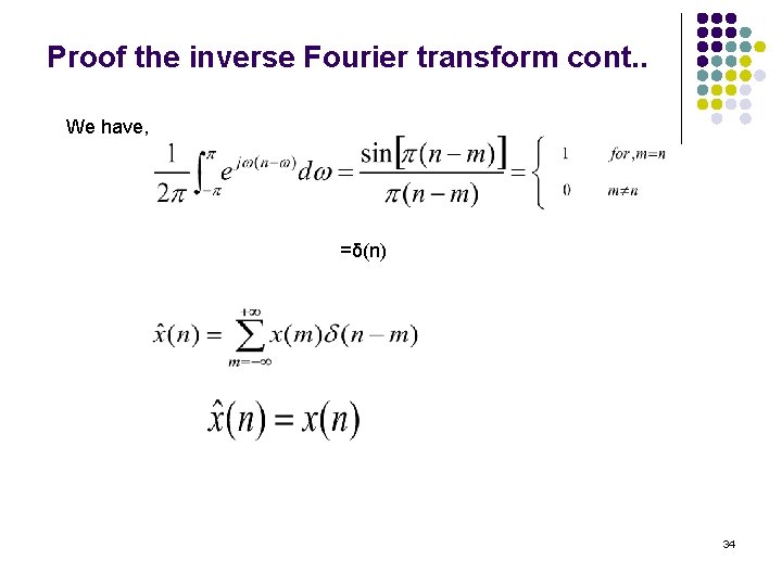
Proof the inverse Fourier transform interchanging the order of integral and summation 33

Proof the inverse Fourier transform cont. . We have, =δ(n) 34

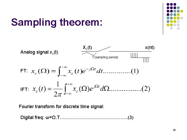
Sampling theorem: Analog signal xc(t) Xc(t) x(nt) T(sampling period) FT: IFT: Fourier transform for discrete time signal: Digital freq: ω=Ω. T…………………. . (3) 35

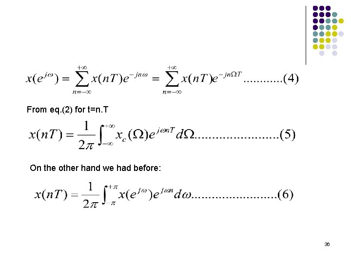
From eq. (2) for t=n. T On the other hand we had before: 36

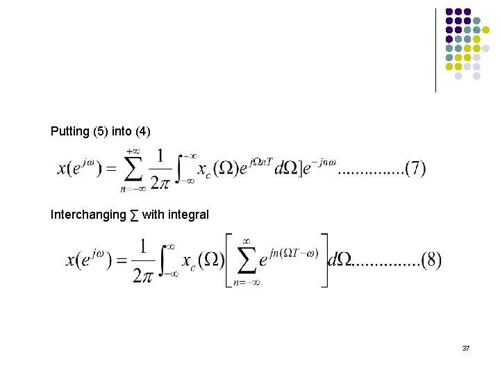
Putting (5) into (4) Interchanging ∑ with integral 37

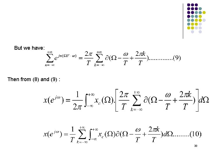
But we have: Then from (8) and (9) : 38

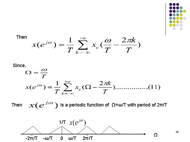
Then Since, Then is a periodic function of Ω=ω/T with period of 2π/T 1/T -2π/T -ω/T 0 ω/T 2π/T Ω 39

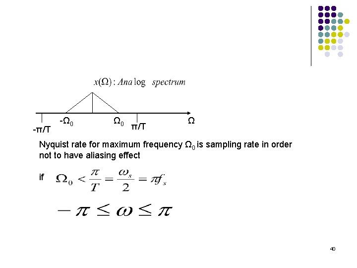
-π/T -Ω 0 π/T Ω Nyquist rate for maximum frequency Ω 0 is sampling rate in order not to have aliasing effect if 40

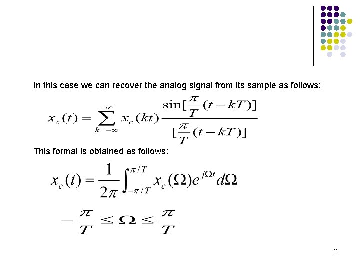
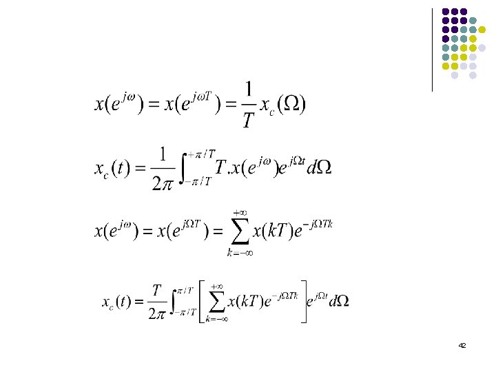
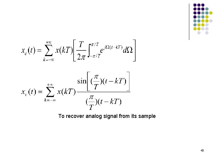
In this case we can recover the analog signal from its sample as follows: This formal is obtained as follows: 41

42

To recover analog signal from its sample 43

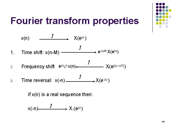
Fourier transform properties x(n) ƒ X(ejω) ƒ 1. Time shift: x(n-M) 2. Frequency shift 3. ƒ ejω0 n x(n) Time reversal: x(-n) e-jωM X(ejω) ƒ X(ej(ω-ω0)) X(e-jω) if x(n) is a real sequence then: x(-n) ƒ X. (ejω) 44

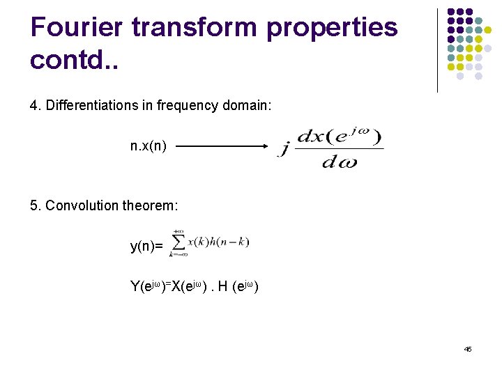
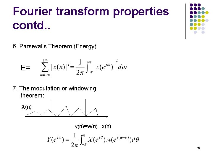
Fourier transform properties contd. . 4. Differentiations in frequency domain: n. x(n) 5. Convolution theorem: y(n)= Y(ejω)=X(ejω). H (ejω) 45

Fourier transform properties contd. . 6. Parseval’s Theorem (Energy) E= 7. The modulation or windowing theorem: X(n) y(n)=w(n). x(n) 46

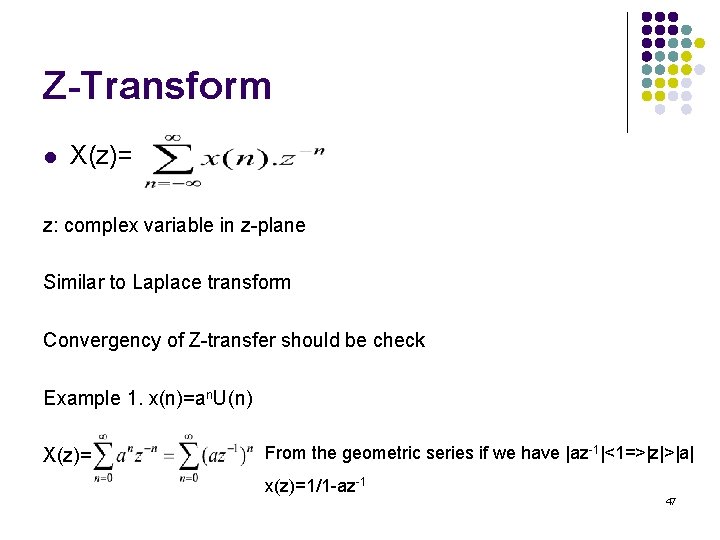
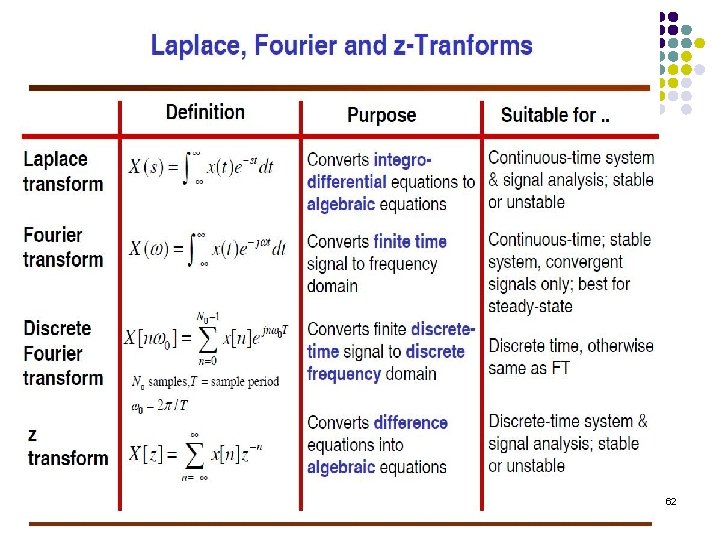
Z-Transform l X(z)= z: complex variable in z-plane Similar to Laplace transform Convergency of Z-transfer should be check Example 1. x(n)=an. U(n) X(z)= From the geometric series if we have |az-1|<1=>|z|>|a| x(z)=1/1 -az-1 47

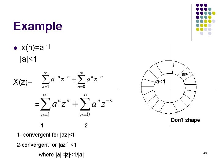
Example l x(n)=a|n| |a|<1 a>1 X(z)= a<1 = 1 2 Don’t shape 1 - convergent for |az|<1 2 -convergent for |az-1|<1 where |a|<|z|<1/|a| 48

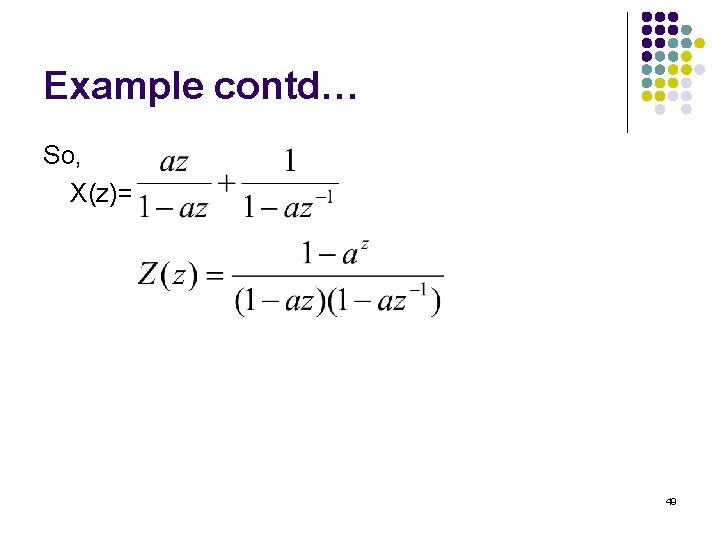
Example contd… So, X(z)= 49

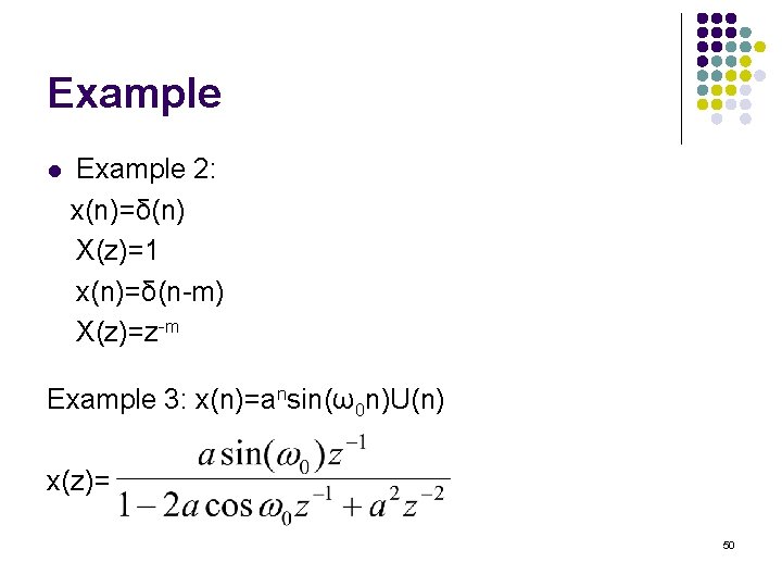
Example l Example 2: x(n)=δ(n) X(z)=1 x(n)=δ(n-m) X(z)=z-m Example 3: x(n)=ansin(ω0 n)U(n) x(z)= 50

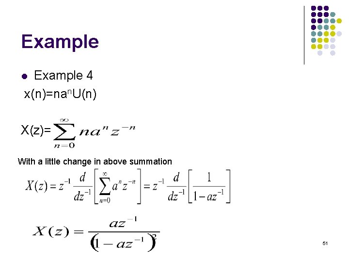
Example 4 x(n)=nan. U(n) l X(z)= With a little change in above summation 51

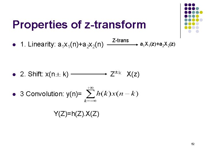
Properties of z-transform l 1. Linearity: a 1 x 1(n)+a 2 x 2(n) l 2. Shift: x(n l 3 Convolution: y(n)= k) Z-trans Z k a 1 X 1(z)+a 2 X 2(z) X(z) Y(Z)=h(Z). X(Z) 52

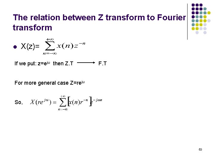
The relation between Z transform to Fourier transform l X(z)= If we put: z=ejω then Z. T For more general case Z=rejω So, 53

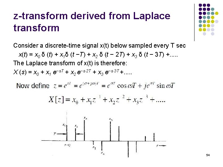
z-transform derived from Laplace transform Consider a discrete-time signal x(t) below sampled every T sec x(t) = x 0 δ (t) + x 1δ (t −T) + x 2 δ (t − 2 T) + x 3 δ (t − 3 T) +. . . The Laplace transform of x(t) is therefore: X (s) = x 0 + x 1 e−s. T + x 2 e−s 2 T + x 3 e−s 3 T +. . . 54

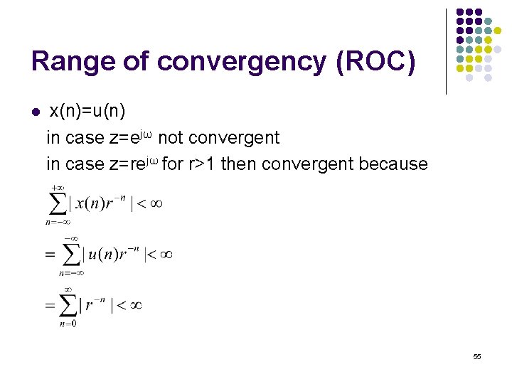
Range of convergency (ROC) l x(n)=u(n) in case z=ejω not convergent in case z=rejω for r>1 then convergent because 55

ROC Contd…. l Step function u(n) has z-transform for ROC: |z|>1 If ROC includes the unit circle then z=ejω and the sequence has Fourier Transform There is possibility that two sequences are different but they may have a similar algebraic form of their z-transform, however their ROC’s are different 56

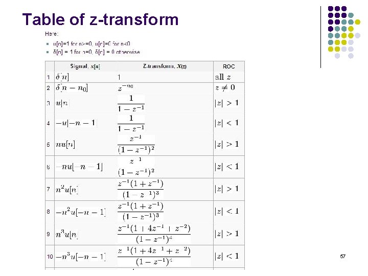
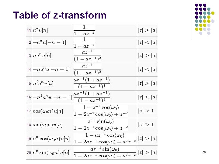
Table of z-transform 57

Table of z-transform 58

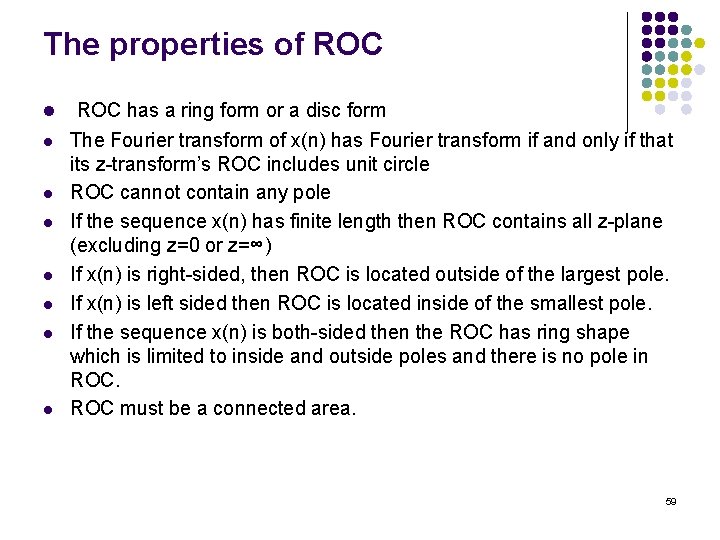
The properties of ROC l l l l ROC has a ring form or a disc form The Fourier transform of x(n) has Fourier transform if and only if that its z-transform’s ROC includes unit circle ROC cannot contain any pole If the sequence x(n) has finite length then ROC contains all z-plane (excluding z=0 or z=∞) If x(n) is right-sided, then ROC is located outside of the largest pole. If x(n) is left sided then ROC is located inside of the smallest pole. If the sequence x(n) is both-sided then the ROC has ring shape which is limited to inside and outside poles and there is no pole in ROC must be a connected area. 59

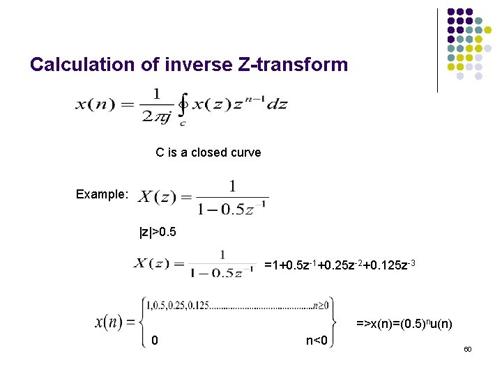
Calculation of inverse Z-transform C is a closed curve Example: |z|>0. 5 =1+0. 5 z-1+0. 25 z-2+0. 125 z-3 =>x(n)=(0. 5)nu(n) 0 n<0 60

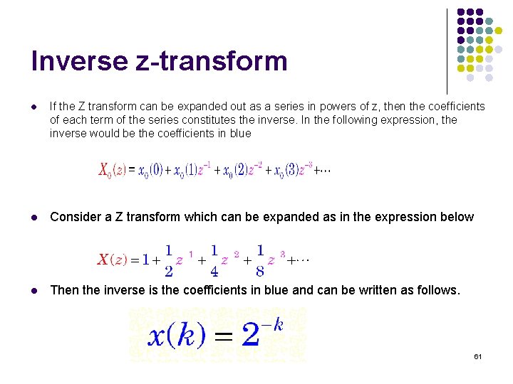
Inverse z-transform l If the Z transform can be expanded out as a series in powers of z, then the coefficients of each term of the series constitutes the inverse. In the following expression, the inverse would be the coefficients in blue l Consider a Z transform which can be expanded as in the expression below l Then the inverse is the coefficients in blue and can be written as follows. 61

62