Sampling and Reconstruction The sampling and reconstruction process

Sampling and Reconstruction The sampling and reconstruction process n Real world: continuous n Digital world: discrete Basic signal processing n Fourier transforms n The convolution theorem n The sampling theorem Aliasing and antialiasing n Uniform supersampling n Nonuniform supersampling CS 348 B Lecture 8 Pat Hanrahan, Spring 2005

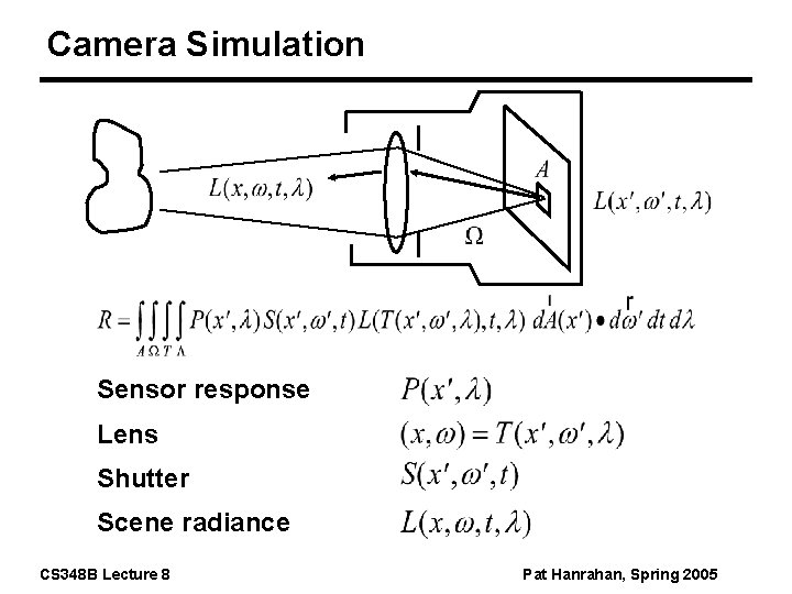
Camera Simulation Sensor response Lens Shutter Scene radiance CS 348 B Lecture 8 Pat Hanrahan, Spring 2005

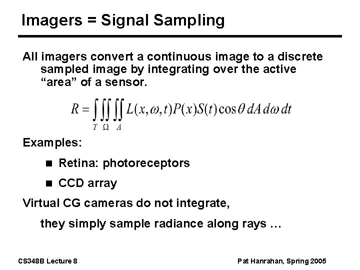
Imagers = Signal Sampling All imagers convert a continuous image to a discrete sampled image by integrating over the active “area” of a sensor. Examples: n Retina: photoreceptors n CCD array Virtual CG cameras do not integrate, they simply sample radiance along rays … CS 348 B Lecture 8 Pat Hanrahan, Spring 2005

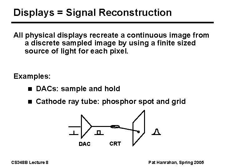
Displays = Signal Reconstruction All physical displays recreate a continuous image from a discrete sampled image by using a finite sized source of light for each pixel. Examples: n DACs: sample and hold n Cathode ray tube: phosphor spot and grid DAC CS 348 B Lecture 8 CRT Pat Hanrahan, Spring 2005

Sampling in Computer Graphics Artifacts due to sampling - Aliasing n Jaggies n Moire n Flickering small objects n Sparkling highlights n Temporal strobing Preventing these artifacts - Antialiasing CS 348 B Lecture 8 Pat Hanrahan, Spring 2005

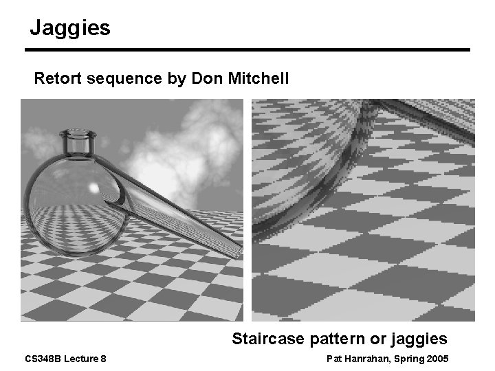
Jaggies Retort sequence by Don Mitchell Staircase pattern or jaggies CS 348 B Lecture 8 Pat Hanrahan, Spring 2005

Basic Signal Processing

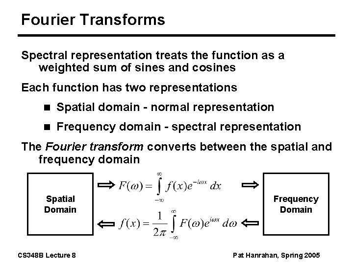
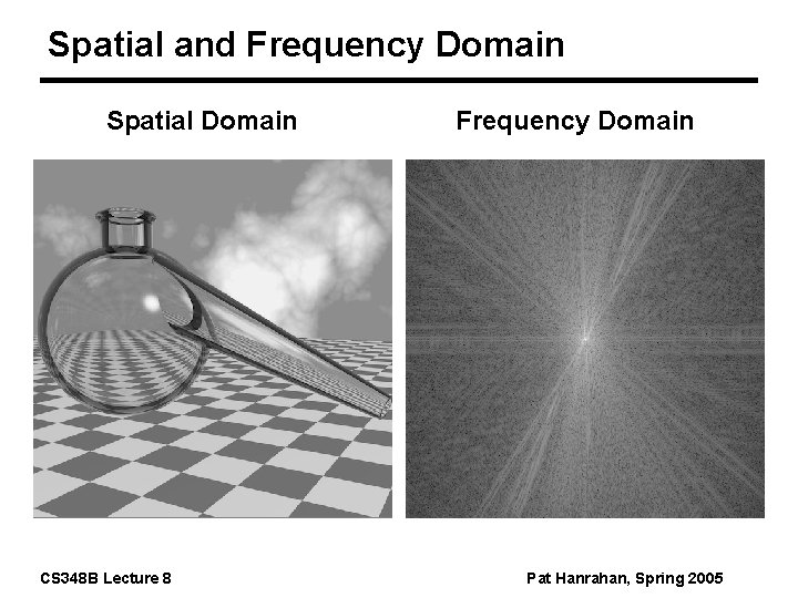
Fourier Transforms Spectral representation treats the function as a weighted sum of sines and cosines Each function has two representations n Spatial domain - normal representation n Frequency domain - spectral representation The Fourier transform converts between the spatial and frequency domain Spatial Domain Frequency Domain CS 348 B Lecture 8 Pat Hanrahan, Spring 2005

Spatial and Frequency Domain Spatial Domain CS 348 B Lecture 8 Frequency Domain Pat Hanrahan, Spring 2005

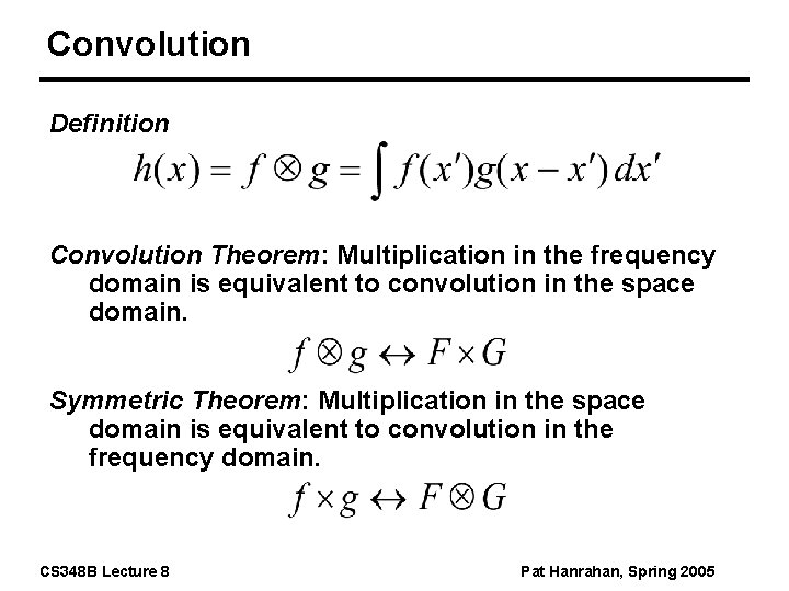
Convolution Definition Convolution Theorem: Multiplication in the frequency domain is equivalent to convolution in the space domain. Symmetric Theorem: Multiplication in the space domain is equivalent to convolution in the frequency domain. CS 348 B Lecture 8 Pat Hanrahan, Spring 2005

The Sampling Theorem

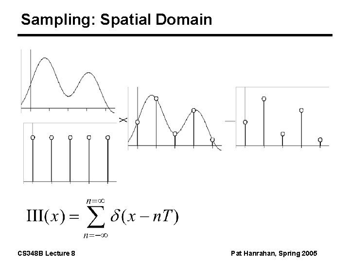
Sampling: Spatial Domain CS 348 B Lecture 8 Pat Hanrahan, Spring 2005

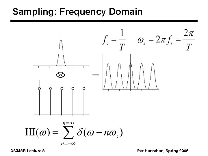
Sampling: Frequency Domain CS 348 B Lecture 8 Pat Hanrahan, Spring 2005

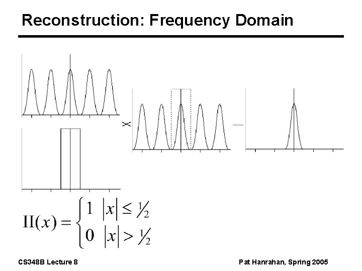
Reconstruction: Frequency Domain CS 348 B Lecture 8 Pat Hanrahan, Spring 2005

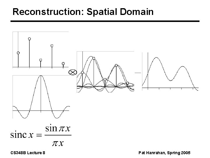
Reconstruction: Spatial Domain CS 348 B Lecture 8 Pat Hanrahan, Spring 2005

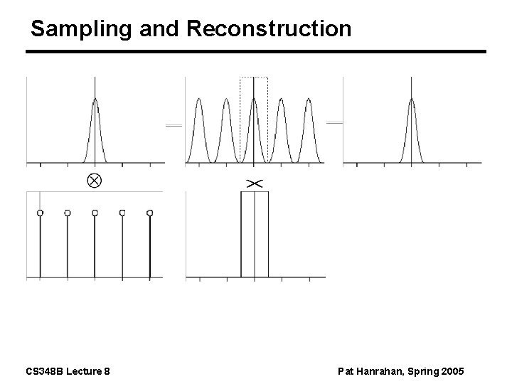
Sampling and Reconstruction CS 348 B Lecture 8 Pat Hanrahan, Spring 2005

Sampling Theorem This result if known as the Sampling Theorem and is due to Claude Shannon who first discovered it in 1949 A signal can be reconstructed from its samples without loss of information, if the original signal has no frequencies above 1/2 the Sampling frequency For a given bandlimited function, the rate at which it must be sampled is called the Nyquist Frequency CS 348 B Lecture 8 Pat Hanrahan, Spring 2005

Aliasing

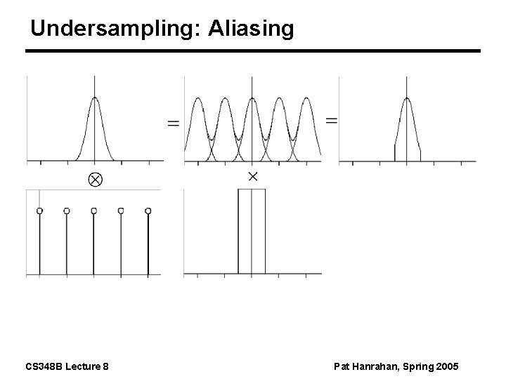
Undersampling: Aliasing CS 348 B Lecture 8 Pat Hanrahan, Spring 2005

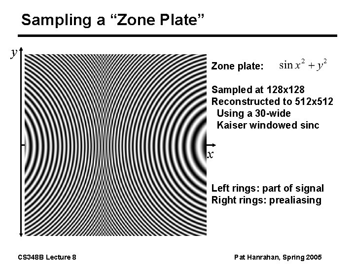
Sampling a “Zone Plate” y Zone plate: Sampled at 128 x 128 Reconstructed to 512 x 512 Using a 30 -wide Kaiser windowed sinc x Left rings: part of signal Right rings: prealiasing CS 348 B Lecture 8 Pat Hanrahan, Spring 2005

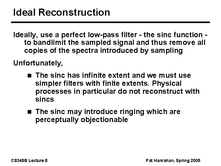
Ideal Reconstruction Ideally, use a perfect low-pass filter - the sinc function to bandlimit the sampled signal and thus remove all copies of the spectra introduced by sampling Unfortunately, n The sinc has infinite extent and we must use simpler filters with finite extents. Physical processes in particular do not reconstruct with sincs n The sinc may introduce ringing which are perceptually objectionable CS 348 B Lecture 8 Pat Hanrahan, Spring 2005

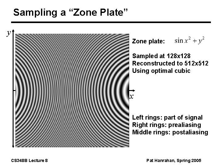
Sampling a “Zone Plate” y Zone plate: Sampled at 128 x 128 Reconstructed to 512 x 512 Using optimal cubic x Left rings: part of signal Right rings: prealiasing Middle rings: postaliasing CS 348 B Lecture 8 Pat Hanrahan, Spring 2005

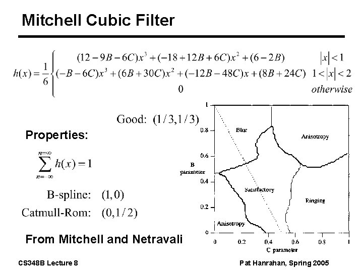
Mitchell Cubic Filter Properties: From Mitchell and Netravali CS 348 B Lecture 8 Pat Hanrahan, Spring 2005

Antialiasing

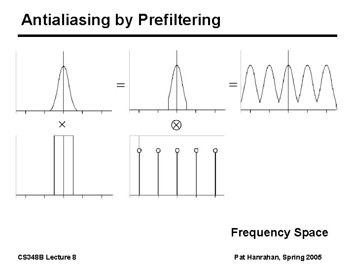
Antialiasing by Prefiltering Frequency Space CS 348 B Lecture 8 Pat Hanrahan, Spring 2005

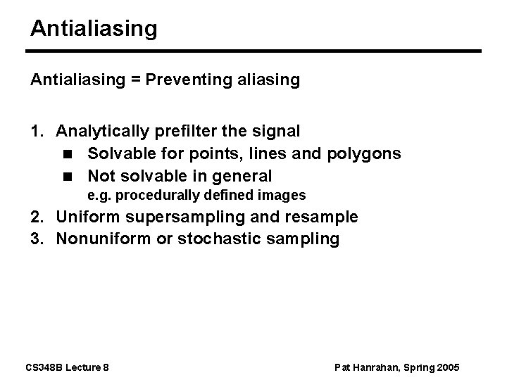
Antialiasing = Preventing aliasing 1. Analytically prefilter the signal n Solvable for points, lines and polygons n Not solvable in general e. g. procedurally defined images 2. Uniform supersampling and resample 3. Nonuniform or stochastic sampling CS 348 B Lecture 8 Pat Hanrahan, Spring 2005

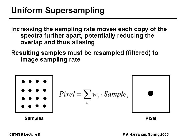
Uniform Supersampling Increasing the sampling rate moves each copy of the spectra further apart, potentially reducing the overlap and thus aliasing Resulting samples must be resampled (filtered) to image sampling rate Samples CS 348 B Lecture 8 Pixel Pat Hanrahan, Spring 2005

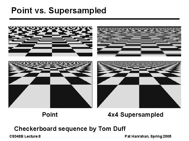
Point vs. Supersampled Point 4 x 4 Supersampled Checkerboard sequence by Tom Duff CS 348 B Lecture 8 Pat Hanrahan, Spring 2005

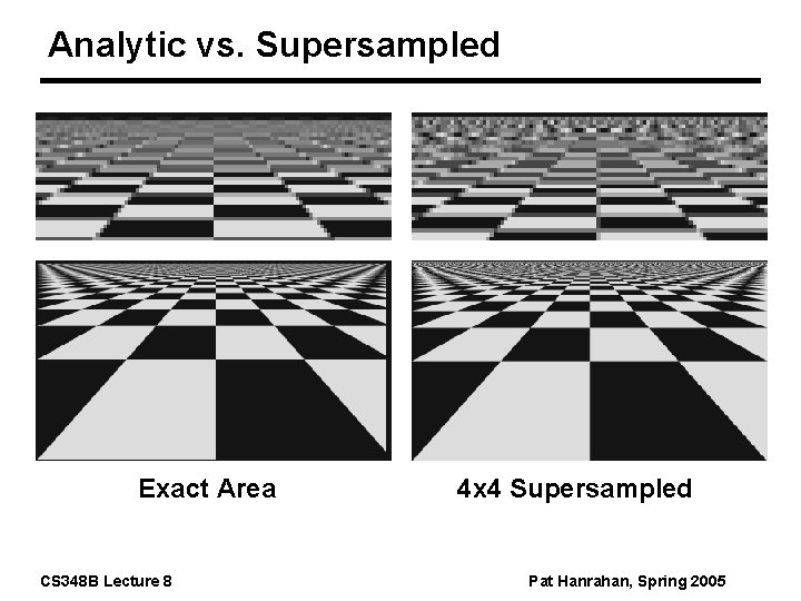
Analytic vs. Supersampled Exact Area CS 348 B Lecture 8 4 x 4 Supersampled Pat Hanrahan, Spring 2005

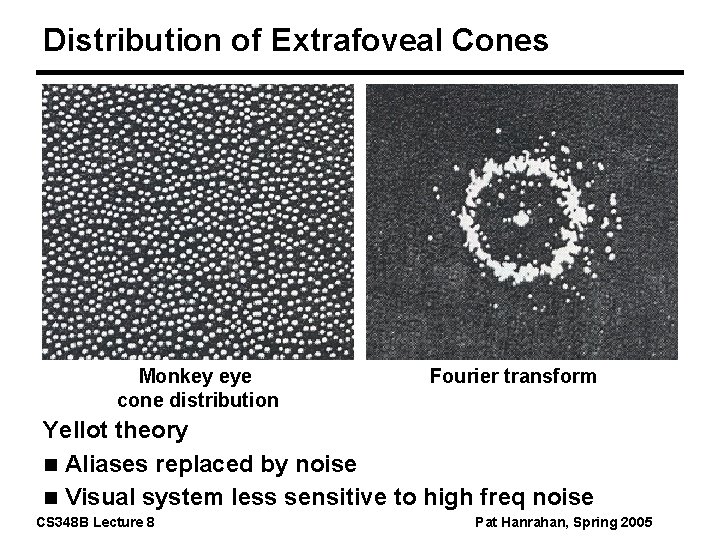
Distribution of Extrafoveal Cones Monkey eye cone distribution Fourier transform Yellot theory n Aliases replaced by noise n Visual system less sensitive to high freq noise CS 348 B Lecture 8 Pat Hanrahan, Spring 2005

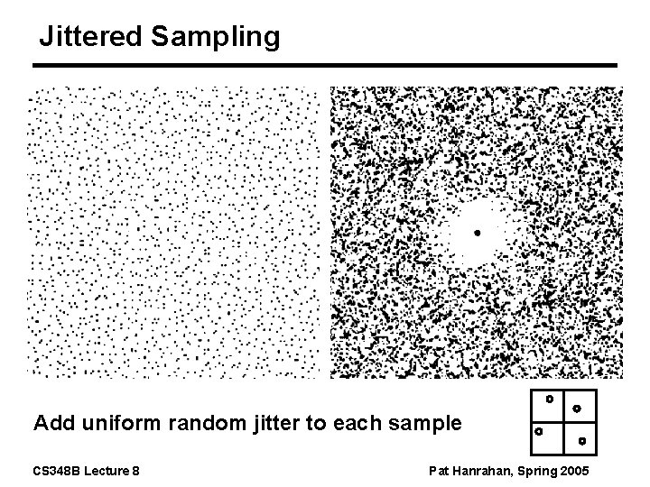
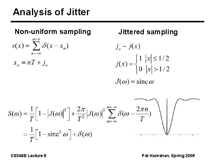
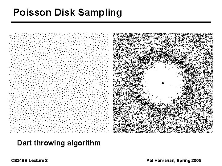
Non-uniform Sampling Intuition Uniform sampling n The spectrum of uniformly spaced samples is also a set of uniformly spaced spikes n Multiplying the signal by the sampling pattern corresponds to placing a copy of the spectrum at each spike (in freq. space) n Aliases are coherent, and very noticable Non-uniform sampling n Samples at non-uniform locations have a different spectrum; a single spike plus noise n Sampling a signal in this way converts aliases into broadband noise n Noise is incoherent, and much less objectionable CS 348 B Lecture 8 Pat Hanrahan, Spring 2005

Jittered Sampling Add uniform random jitter to each sample CS 348 B Lecture 8 Pat Hanrahan, Spring 2005

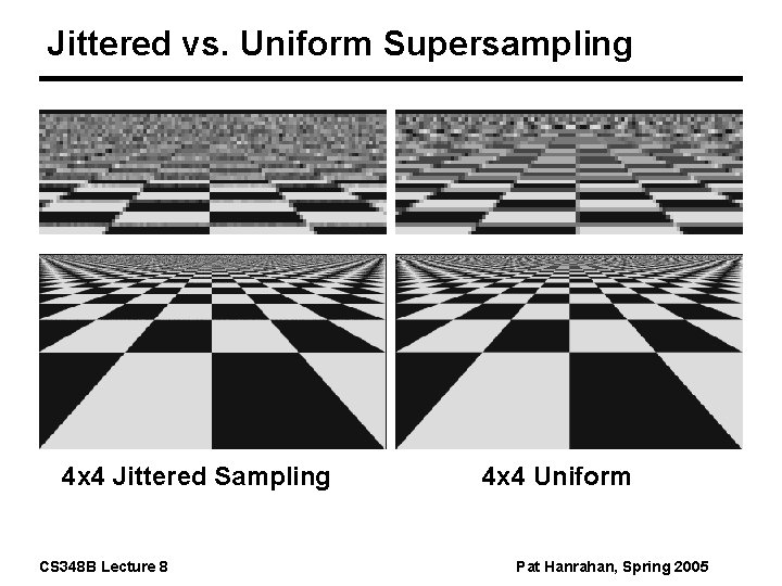
Jittered vs. Uniform Supersampling 4 x 4 Jittered Sampling CS 348 B Lecture 8 4 x 4 Uniform Pat Hanrahan, Spring 2005

Analysis of Jitter Non-uniform sampling CS 348 B Lecture 8 Jittered sampling Pat Hanrahan, Spring 2005

Poisson Disk Sampling Dart throwing algorithm CS 348 B Lecture 8 Pat Hanrahan, Spring 2005