RNASeq and Transcriptome Analysis Jessica Holmes High Performance

RNA-Seq and Transcriptome Analysis Jessica Holmes High Performance Biological Computing (HPCBio) Roy J. Carver Biotechnology Center

General Outline 1. Getting the RNA-Seq data: from RNA -> Sequence data 2. Experimental and practical considerations 3. Commonly encountered file formats 4. Transcriptomic analysis methods and tools a. Transcriptome Assembly b. Differential Gene expression

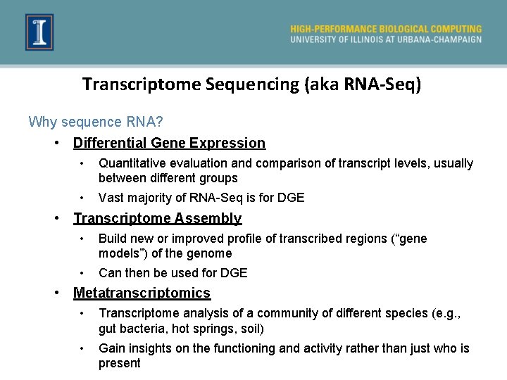
Transcriptome Sequencing (aka RNA-Seq) Why sequence RNA? • Differential Gene Expression • Quantitative evaluation and comparison of transcript levels, usually between different groups • Vast majority of RNA-Seq is for DGE • Transcriptome Assembly • Build new or improved profile of transcribed regions (“gene models”) of the genome • Can then be used for DGE • Metatranscriptomics • Transcriptome analysis of a community of different species (e. g. , gut bacteria, hot springs, soil) • Gain insights on the functioning and activity rather than just who is present

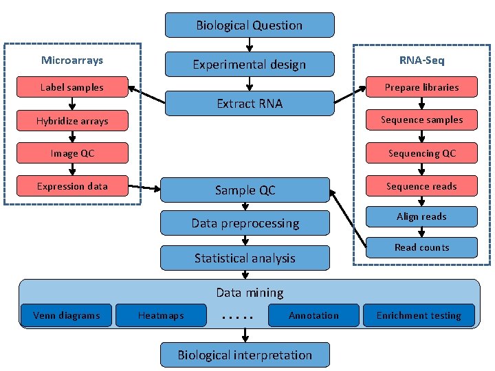
Biological Question Microarrays Experimental design Label samples RNA-Seq Prepare libraries Extract RNA Hybridize arrays Sequence samples Image QC Sequencing QC Expression data Sample QC Sequence reads Data preprocessing Align reads Statistical analysis Read counts Data mining Venn diagrams Heatmaps …. . Annotation Biological interpretation Enrichment testing

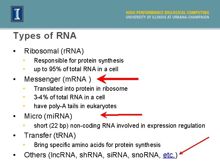
Types of RNA • Ribosomal (r. RNA) • • • Messenger (m. RNA ) • • short (22 bp) non-coding RNA involved in expression regulation Transfer (t. RNA) • • Translated into protein in ribosome 3 -4% of total RNA in a cell have poly-A tails in eukaryotes Micro (mi. RNA) • • Responsible for protein synthesis up to 95% of total RNA in a cell Bring specific amino acids for protein synthesis Others (lnc. RNA, sh. RNA, si. RNA, sno. RNA, etc. )

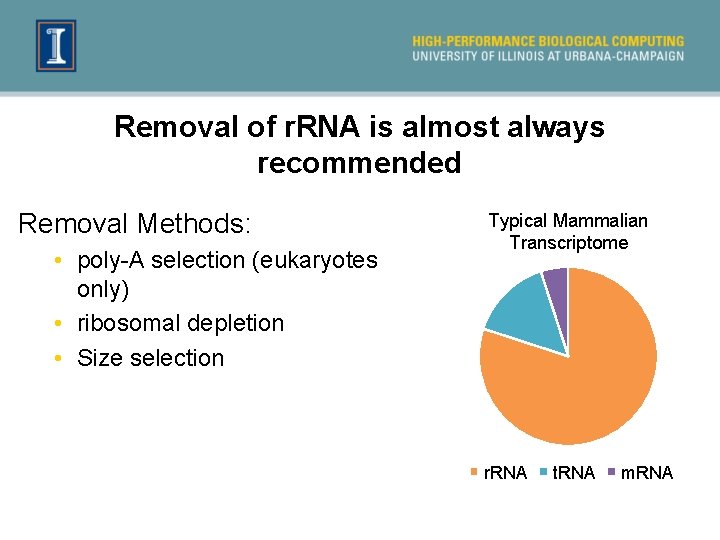
Removal of r. RNA is almost always recommended Removal Methods: • poly-A selection (eukaryotes only) • ribosomal depletion • Size selection Typical Mammalian Transcriptome r. RNA t. RNA m. RNA

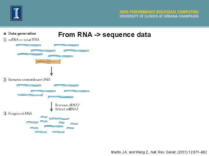
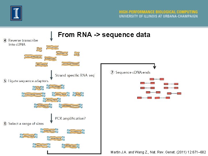
From RNA -> sequence data Martin J. A. and Wang Z. , Nat. Rev. Genet. (2011) 12: 671– 682

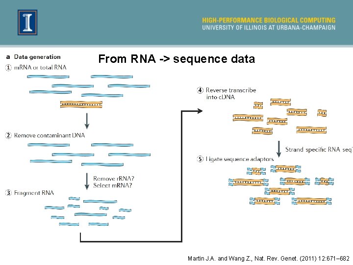
From RNA -> sequence data Martin J. A. and Wang Z. , Nat. Rev. Genet. (2011) 12: 671– 682

From RNA -> sequence data Martin J. A. and Wang Z. , Nat. Rev. Genet. (2011) 12: 671– 682

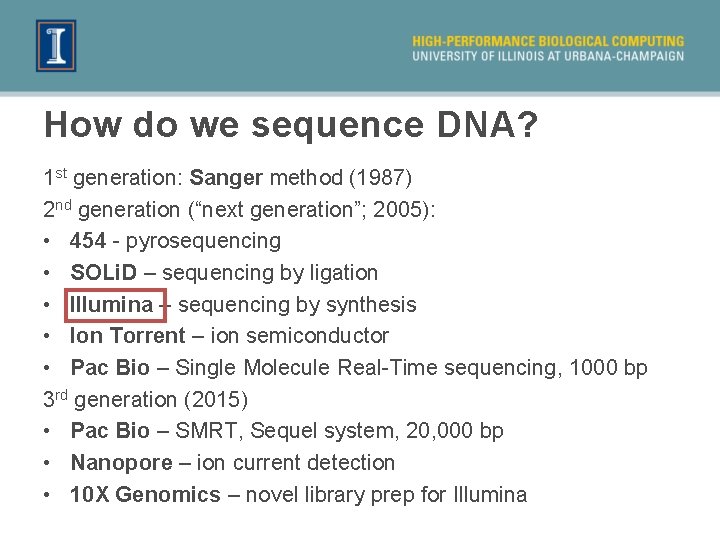
How do we sequence DNA? 1 st generation: Sanger method (1987) 2 nd generation (“next generation”; 2005): • 454 - pyrosequencing • SOLi. D – sequencing by ligation • Illumina – sequencing by synthesis • Ion Torrent – ion semiconductor • Pac Bio – Single Molecule Real-Time sequencing, 1000 bp 3 rd generation (2015) • Pac Bio – SMRT, Sequel system, 20, 000 bp • Nanopore – ion current detection • 10 X Genomics – novel library prep for Illumina

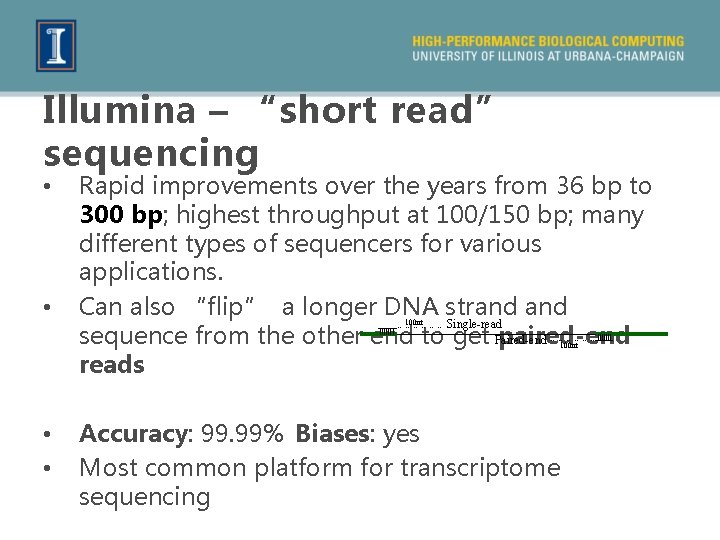
Illumina – “short read” sequencing • • Rapid improvements over the years from 36 bp to 300 bp; highest throughput at 100/150 bp; many different types of sequencers for various applications. Can also “flip” a longer DNA strand Single-read sequence from the other end to get Paired-end paired-end reads 100 nt ……………. . 100 nt • • Accuracy: 99. 99% Biases: yes Most common platform for transcriptome sequencing

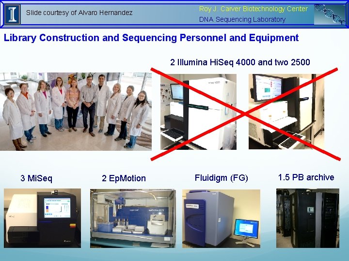
Slide courtesy of Alvaro Hernandez Roy J. Carver Biotechnology Center DNA Sequencing Laboratory Library Construction and Sequencing Personnel and Equipment 2 Illumina Hi. Seq 4000 and two 2500 3 Mi. Seq 2 Ep. Motion Fluidigm (FG) 1. 5 PB archive

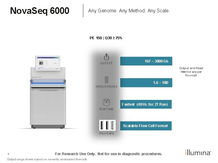
Nova. Seq 6000 Any Genome. Any Method. Any Scale. PE 150 | Q 30 ≥ 75% OUTPUT 167 – 3000 Gb Output and Read Metrics are per flow cell 1. 6 – 10 B SINGLE READS Fastest (40 Hr. for 2 T Run) RUN TIME Scalable Flow Cell Format Flow Cells 6 For Research Use Only. Not for use in diagnostic procedures. Output range shown based on currently unreleased flow cells

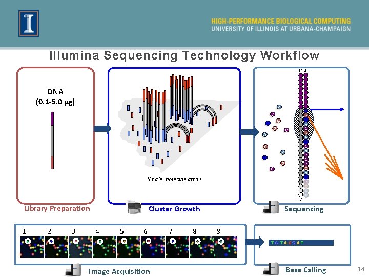
Illumina Sequencing Technology Workflow 3’ 5’ DNA (0. 1 -5. 0 μg) A T C C G G C A G A T G C Single molecule array 5’ Library Preparation 1 2 3 Sequencing Cluster Growth 4 5 6 7 8 T G T A C G A T C A C C C G A T C G A A 9 TG TACGAT… Image Acquisition Base Calling 14

Illumina Sequencing Video Introduction to Sequencing by Synthesis

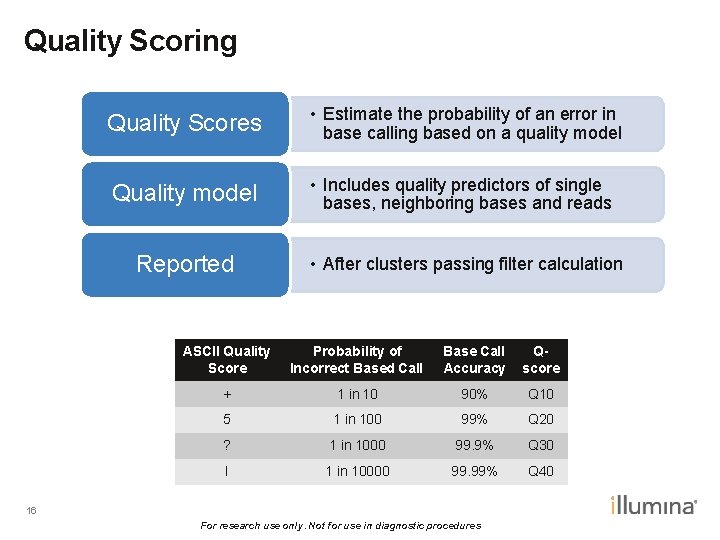
Quality Scoring Quality Scores • Estimate the probability of an error in base calling based on a quality model Quality model • Includes quality predictors of single bases, neighboring bases and reads Reported • After clusters passing filter calculation ASCII Quality Score Probability of Incorrect Based Call Base Call Accuracy Qscore + 1 in 10 90% Q 10 5 1 in 100 99% Q 20 ? 1 in 1000 99. 9% Q 30 I 1 in 10000 99. 99% Q 40 16 For research use only. Not for use in diagnostic procedures

General Outline 1. Getting the RNA-Seq data: from RNA -> Sequence data 2. Experimental and Practical considerations 3. Commonly encountered file formats 4. Transcriptomic analysis methods and tools a. Transcriptome Assembly b. Differential Gene expression

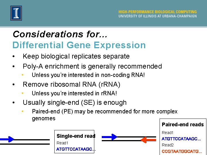
Considerations for. . . Differential Gene Expression • • Keep biological replicates separate Poly-A enrichment is generally recommended • • Remove ribosomal RNA (r. RNA) • • Unless you’re interested in non-coding RNA! Unless you’re interested in r. RNA! Usually single-end (SE) is enough • Paired-end (PE) may be recommended for more complex genomes Paired-end reads Single-end read Read 1 ATGTTCCATAAGC… Read 2 CCGTAATGGCATG…

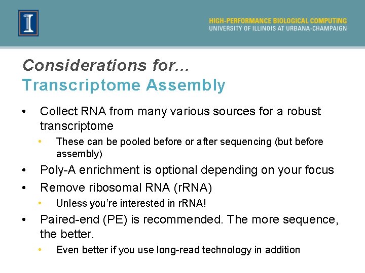
Considerations for. . . Transcriptome Assembly • Collect RNA from many various sources for a robust transcriptome • • • Poly-A enrichment is optional depending on your focus Remove ribosomal RNA (r. RNA) • • These can be pooled before or after sequencing (but before assembly) Unless you’re interested in r. RNA! Paired-end (PE) is recommended. The more sequence, the better. • Even better if you use long-read technology in addition

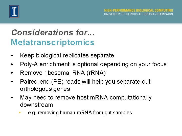
Considerations for. . . Metatranscriptomics • • • Keep biological replicates separate Poly-A enrichment is optional depending on your focus Remove ribosomal RNA (r. RNA) Paired-end (PE) reads will help you separate out orthologous genes May need to remove host m. RNA computationally downstream • e. g. removing human m. RNA from gut samples

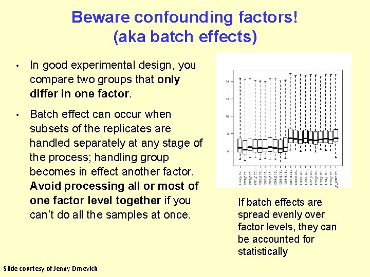
Beware confounding factors! (aka batch effects) • In good experimental design, you compare two groups that only differ in one factor. • Batch effect can occur when subsets of the replicates are handled separately at any stage of the process; handling group becomes in effect another factor. Avoid processing all or most of one factor level together if you can’t do all the samples at once. Slide courtesy of Jenny Drnevich If batch effects are spread evenly over factor levels, they can be accounted for statistically

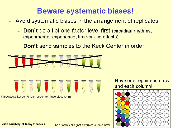
Beware systematic biases! • Avoid systematic biases in the arrangement of replicates. – Don’t do all of one factor level first (circadian rhythms, experimenter experience, time-on-ice effects) – Don’t send samples to the Keck Center in order Have one rep in each row and each column! http: //www. clker. com/clipart-eppendorf-tube-closed. html Slide courtesy of Jenny Drnevich http: //www. cellsignet. com/media/templ. html

General Outline 1. Getting the RNA-Seq data: from RNA -> Sequence data 2. Experimental and Practical considerations 3. Commonly encountered file formats 4. Transcriptomic analysis methods and tools a. Transcriptome Assembly b. Differential Gene expression

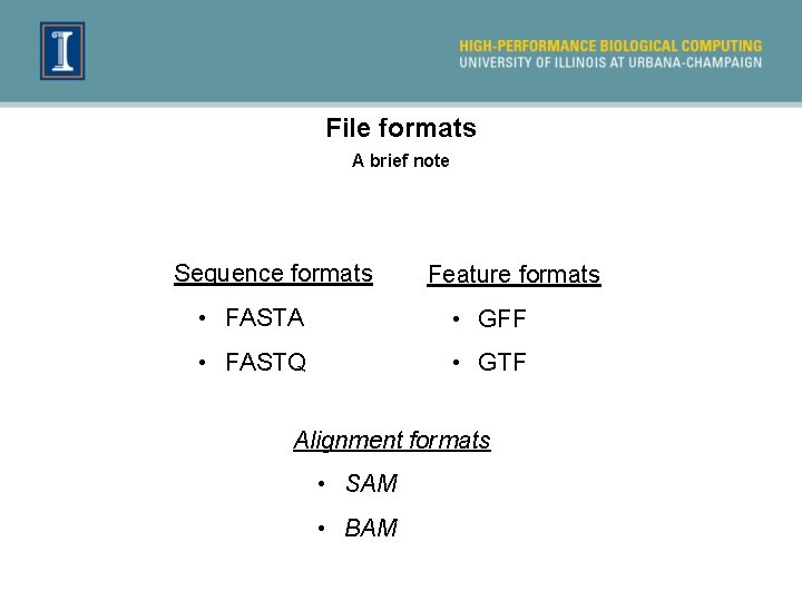
File formats A brief note Sequence formats Feature formats • FASTA • GFF • FASTQ • GTF Alignment formats • SAM • BAM

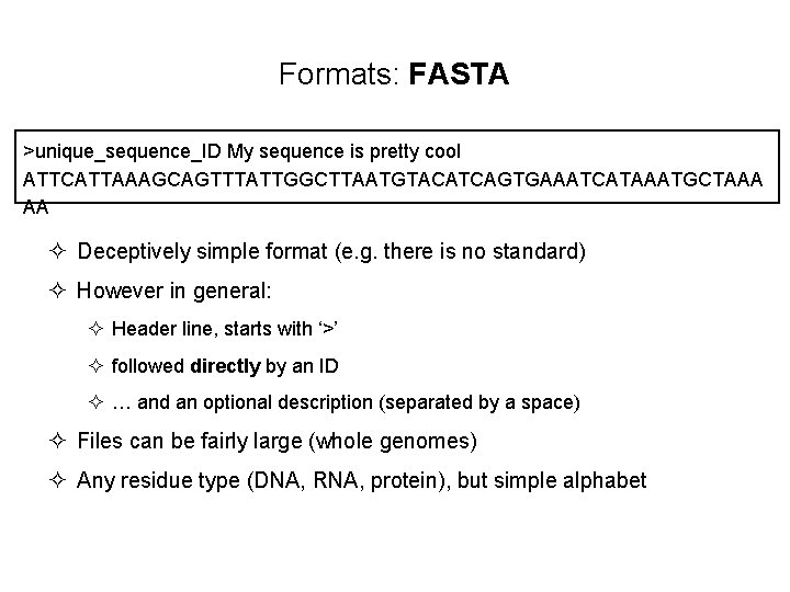
Formats: FASTA >unique_sequence_ID My sequence is pretty cool ATTCATTAAAGCAGTTTATTGGCTTAATGTACATCAGTGAAATCATAAATGCTAAA AA ² Deceptively simple format (e. g. there is no standard) ² However in general: ² Header line, starts with ‘>’ ² followed directly by an ID ² … and an optional description (separated by a space) ² Files can be fairly large (whole genomes) ² Any residue type (DNA, RNA, protein), but simple alphabet

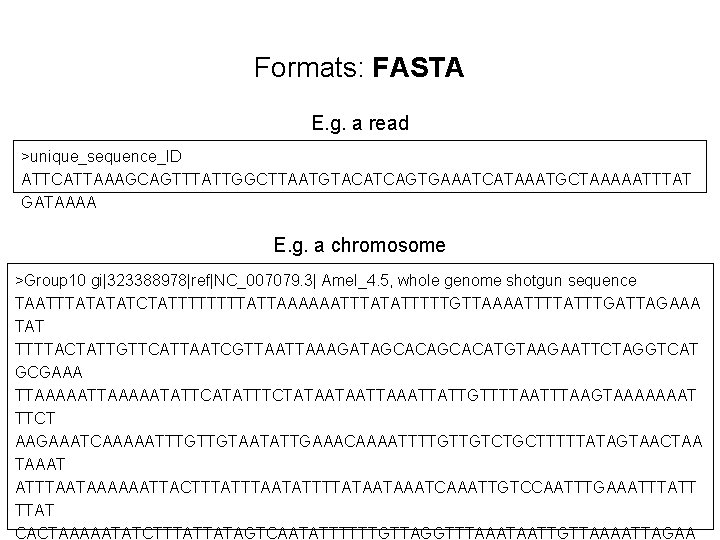
Formats: FASTA E. g. a read >unique_sequence_ID ATTCATTAAAGCAGTTTATTGGCTTAATGTACATCAGTGAAATCATAAATGCTAAAAATTTAT GATAAAA E. g. a chromosome >Group 10 gi|323388978|ref|NC_007079. 3| Amel_4. 5, whole genome shotgun sequence TAATTTATATATCTATTTTATTAAAAAATTTATATTTTTGTTAAAATTTTATTTGATTAGAAA TAT TTTTACTATTGTTCATTAATCGTTAAAGATAGCACATGTAAGAATTCTAGGTCAT GCGAAA TTAAAAATATTCATATTTCTATAATAATTATTGTTTTAAGTAAAAAAAT TTCT AAGAAATCAAAAATTTGTTGTAATATTGAAACAAAATTTTGTTGTCTGCTTTTTATAGTAACTAA TAAAT ATTTAATAAAAAATTACTTTAATATTTTATAATAAATCAAATTGTCCAATTTGAAATTTATT TTAT CACTAAAAATATCTTTATTATAGTCAATATTTTTTGTTAGGTTTAAATAATTGTTAAAATTAGAA

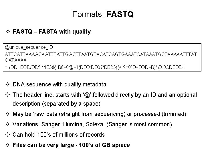
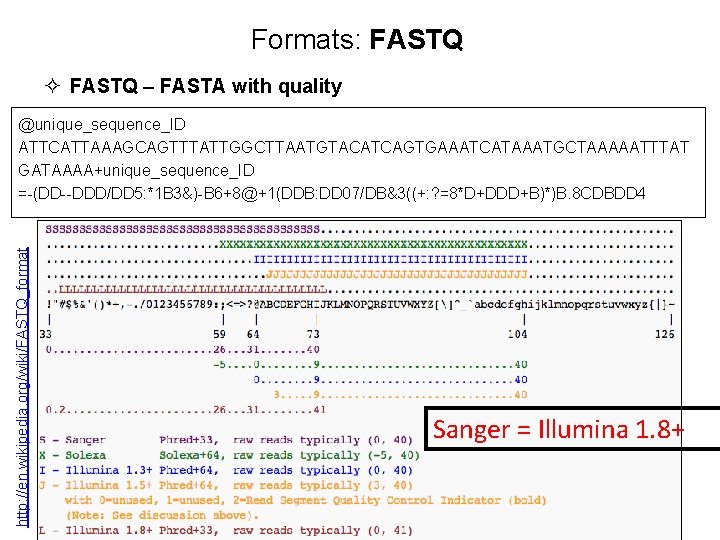
Formats: FASTQ ² FASTQ – FASTA with quality @unique_sequence_ID ATTCATTAAAGCAGTTTATTGGCTTAATGTACATCAGTGAAATCATAAATGCTAAAAATTTAT GATAAAA+ =-(DD--DDD/DD 5: *1 B 3&)-B 6+8@+1(DDB: DD 07/DB&3((+: ? =8*D+DDD+B)*)B. 8 CDBDD 4 ² DNA sequence with quality metadata ² The header line, starts with ‘@’, followed directly by an ID and an optional description (separated by a space) ² May be ‘raw’ data (straight from sequencing) or processed (trimmed) ² Variations: Sanger, Illumina, Solexa (Sanger is most common) ² Can hold 100’s of millions of records ² Files can be very large - 100’s of GB apiece

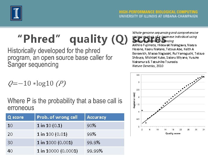
Whole-genome sequencing and comprehensive variant analysis of a Japanese individual using massively parallel sequencing Akihiro Fujimoto, Hidewaki Nakagawa, Naoya Hosono, Kaoru Nakano, Tetsuo Abe, Keith A Boroevich, Masao Nagasaki, Rui Yamaguchi, Tetsuo Shibuya, Michiaki Kubo, Satoru Miyano, Yusuke Nakamura & Tatsuhiko Tsunoda Nature Genetics, 2010 “Phred” quality (Q) scores Q score Prob. of wrong call Accuracy 10 1 in 10 (0. 1) 90% 20 1 in 100 (0. 01) 99% 30 1 in 1000 (0. 001) 99. 9% 40 1 in 10000 (0. 0001) 99. 99%

Formats: FASTQ ² FASTQ – FASTA with quality http: //en. wikipedia. org/wiki/FASTQ_format @unique_sequence_ID ATTCATTAAAGCAGTTTATTGGCTTAATGTACATCAGTGAAATCATAAATGCTAAAAATTTAT GATAAAA+unique_sequence_ID =-(DD--DDD/DD 5: *1 B 3&)-B 6+8@+1(DDB: DD 07/DB&3((+: ? =8*D+DDD+B)*)B. 8 CDBDD 4 Sanger = Illumina 1. 8+

Feature formats ² GTF/GFF 3 ² SAM/BAM ² UCSC formats (BED, WIG, etc. )

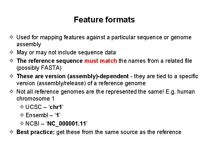
Feature formats ² Used for mapping features against a particular sequence or genome assembly ² May or may not include sequence data ² The reference sequence must match the names from a related file (possibly FASTA) ² These are version (assembly)-dependent - they are tied to a specific version (assembly/release) of a reference genome ² Not all reference genomes are the represented the same! E. g. human chromosome 1 ² UCSC – ‘chr 1’ ² Ensembl – ‘ 1’ ² NCBI – ‘NC_000001. 11’ ² Best practice: get these from the same source as the reference

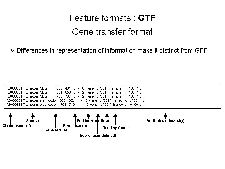
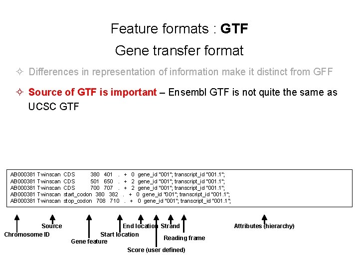
Feature formats : GTF Gene transfer format ² Differences in representation of information make it distinct from GFF AB 000381 Twinscan CDS 380 401 . + 0 gene_id "001"; transcript_id "001. 1"; AB 000381 Twinscan CDS 501 650 . + 2 gene_id "001"; transcript_id "001. 1"; AB 000381 Twinscan CDS 700 707 . + 2 gene_id "001"; transcript_id "001. 1"; AB 000381 Twinscan start_codon 380 382 . + 0 gene_id "001"; transcript_id "001. 1"; AB 000381 Twinscan stop_codon 708 710 . + 0 gene_id "001"; transcript_id "001. 1"; Source Chromosome ID End location Strand Start location Reading frame Gene feature Score (user defined) Attributes (hierarchy)

Feature formats : GTF Gene transfer format ² Differences in representation of information make it distinct from GFF ² Source of GTF is important – Ensembl GTF is not quite the same as UCSC GTF AB 000381 Twinscan CDS 380 401 . + 0 gene_id "001"; transcript_id "001. 1"; AB 000381 Twinscan CDS 501 650 . + 2 gene_id "001"; transcript_id "001. 1"; AB 000381 Twinscan CDS 700 707 . + 2 gene_id "001"; transcript_id "001. 1"; AB 000381 Twinscan start_codon 380 382 . + 0 gene_id "001"; transcript_id "001. 1"; AB 000381 Twinscan stop_codon 708 710 . + 0 gene_id "001"; transcript_id "001. 1"; Source Chromosome ID End location Strand Start location Reading frame Gene feature Score (user defined) Attributes (hierarchy)

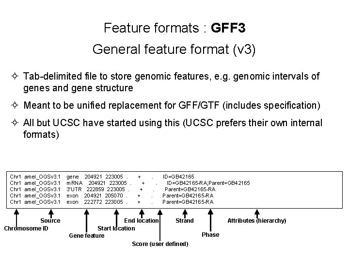
Feature formats : GFF 3 General feature format (v 3) ² Tab-delimited file to store genomic features, e. g. genomic intervals of genes and gene structure ² Meant to be unified replacement for GFF/GTF (includes specification) ² All but UCSC have started using this (UCSC prefers their own internal formats) Chr 1 amel_OGSv 3. 1 gene 204921 223005 . + . ID=GB 42165 Chr 1 amel_OGSv 3. 1 m. RNA 204921 223005 . + . ID=GB 42165 -RA; Parent=GB 42165 Chr 1 amel_OGSv 3. 1 3’UTR 222859 223005 . + . Parent=GB 42165 -RA Chr 1 amel_OGSv 3. 1 exon 204921 205070 . + . Parent=GB 42165 -RA Chr 1 amel_OGSv 3. 1 exon 222772 223005 . + . Parent=GB 42165 -RA Source Chromosome ID End location Strand Start location Gene feature Score (user defined) Attributes (hierarchy) Phase

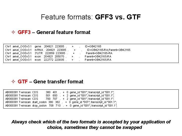
Feature formats: GFF 3 vs. GTF ² GFF 3 – General feature format Chr 1 amel_OGSv 3. 1 gene 204921 223005 . + . ID=GB 42165 Chr 1 amel_OGSv 3. 1 m. RNA 204921 223005 . + . ID=GB 42165 -RA; Parent=GB 42165 Chr 1 amel_OGSv 3. 1 3’UTR 222859 223005 . + . Parent=GB 42165 -RA Chr 1 amel_OGSv 3. 1 exon 204921 205070 . + . Parent=GB 42165 -RA Chr 1 amel_OGSv 3. 1 exon 222772 223005 . + . Parent=GB 42165 -RA ² GTF – Gene transfer format AB 000381 Twinscan CDS 380 401 . + 0 gene_id "001"; transcript_id "001. 1"; AB 000381 Twinscan CDS 501 650 . + 2 gene_id "001"; transcript_id "001. 1"; AB 000381 Twinscan CDS 700 707 . + 2 gene_id "001"; transcript_id "001. 1"; AB 000381 Twinscan start_codon 380 382 . + 0 gene_id "001"; transcript_id "001. 1"; AB 000381 Twinscan stop_codon 708 710 . + 0 gene_id "001"; transcript_id "001. 1"; Always check which of the two formats is accepted by your application of choice, sometimes they cannot be swapped

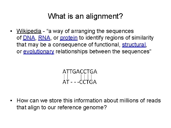
What is an alignment? • Wikipedia - “a way of arranging the sequences of DNA, RNA, or protein to identify regions of similarity that may be a consequence of functional, structural, or evolutionary relationships between the sequences” • How can we store this information about millions of reads that align to our reference genome?

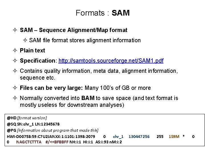
Formats : SAM ² SAM – Sequence Alignment/Map format ² SAM file format stores alignment information ² Plain text ² Specification: http: //samtools. sourceforge. net/SAM 1. pdf ² Contains quality information, meta data, alignment information, sequence etc. ² Files can be very large: Many 100’s of GB or more ² Normally converted into BAM to save space (and text format is mostly useless for downstream analyses) @HD[format version] @SQ SN: chr_1 LN: 12345678 @PG [information about program that made this] HWI-D 00758: 59: C 7 U 2 JANXX: 1: 1101: 1398: 2079 0 chr_1 0 NAGCTCTTTA #/<<BFBBFF NH: i: 1 HI: i: 1 AS: i: 93 n. M: i: 2 130447256 255 1 S 9 M * 0

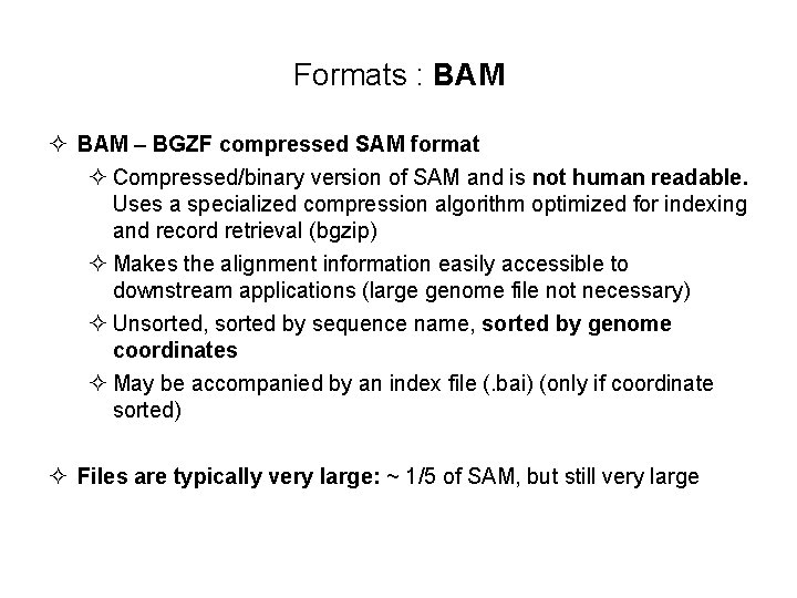
Formats : BAM ² BAM – BGZF compressed SAM format ² Compressed/binary version of SAM and is not human readable. Uses a specialized compression algorithm optimized for indexing and record retrieval (bgzip) ² Makes the alignment information easily accessible to downstream applications (large genome file not necessary) ² Unsorted, sorted by sequence name, sorted by genome coordinates ² May be accompanied by an index file (. bai) (only if coordinate sorted) ² Files are typically very large: ~ 1/5 of SAM, but still very large

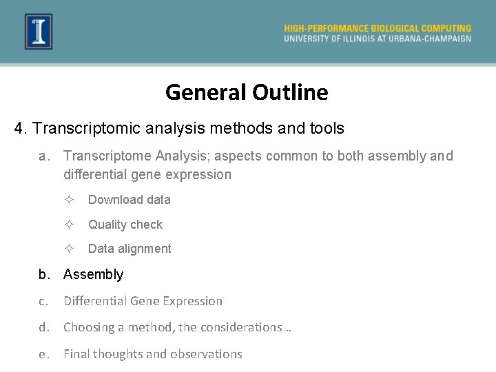
General Outline 4. Transcriptomic analysis methods and tools a. Transcriptome Analysis; aspects common to both assembly and differential gene expression ² Download data ² Quality check ² Data alignment b. Assembly c. Differential Gene Expression d. Choosing a method, the considerations… e. Final thoughts and observations

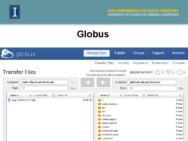
Obtain sequence data 1. If you are using the R. J. C. Biotechnology Center and the Biocluster ² Globus is most direct route ² CNRG instructions 2. Download data to a computer and upload to Biocluster using an SFTP client ² Cyberduck, Win. SCP… 3. Can also use linux commands such as: ² scp, rsync, wget, …

Globus

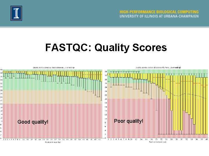
So how can we check the quality of our raw sequences? Software called FASTQC • Name is a play on FASTQ format and QC (Quality Control) • Checks quality by several metrics, and creates a visual report

FASTQC: Quality Scores Good quality! Poor quality!

FASTQC cont. . . Additional metrics • • Presence of, and abundance of contaminating sequences Average read length GC content And more! Assumes that your data is: • WGS (i. e. evenish sampling of the whole genome) • Derived from DNA • Derived from one species So keep this in mind when interpreting results

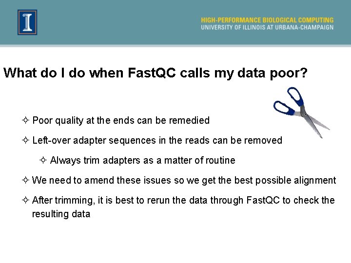
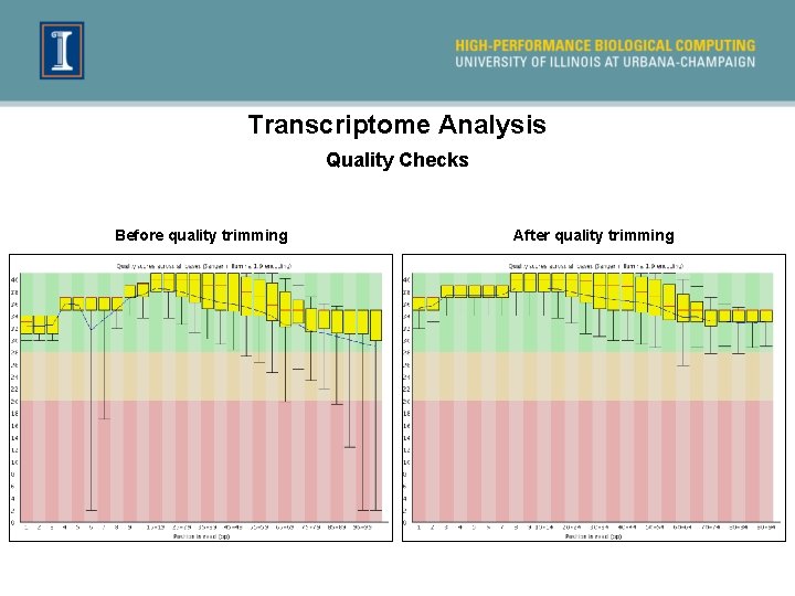
What do I do when Fast. QC calls my data poor? ² Poor quality at the ends can be remedied ² Left-over adapter sequences in the reads can be removed ² Always trim adapters as a matter of routine ² We need to amend these issues so we get the best possible alignment ² After trimming, it is best to rerun the data through Fast. QC to check the resulting data

Transcriptome Analysis Quality Checks Before quality trimming After quality trimming

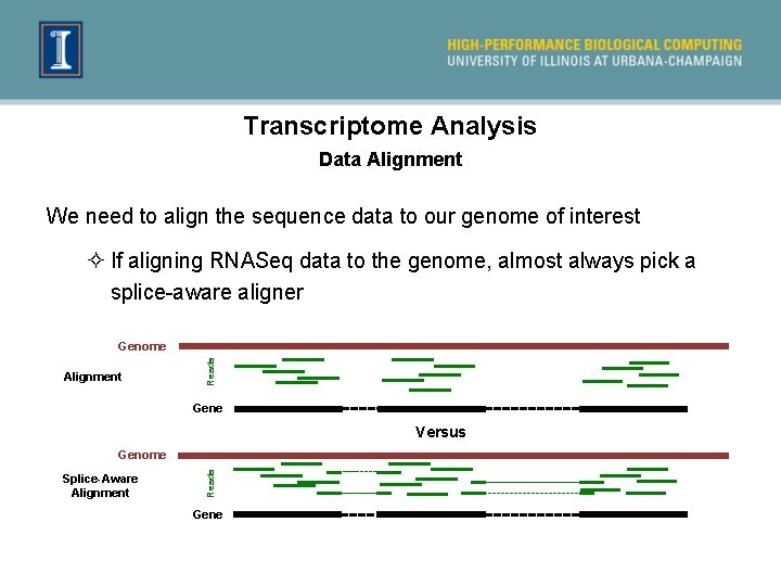
Transcriptome Analysis Data Alignment We need to align the sequence data to our genome of interest ² If aligning RNASeq data to the genome, almost always pick a splice-aware aligner Alignment Reads Genome Gene Versus Splice-Aware Alignment Reads Genome Gene

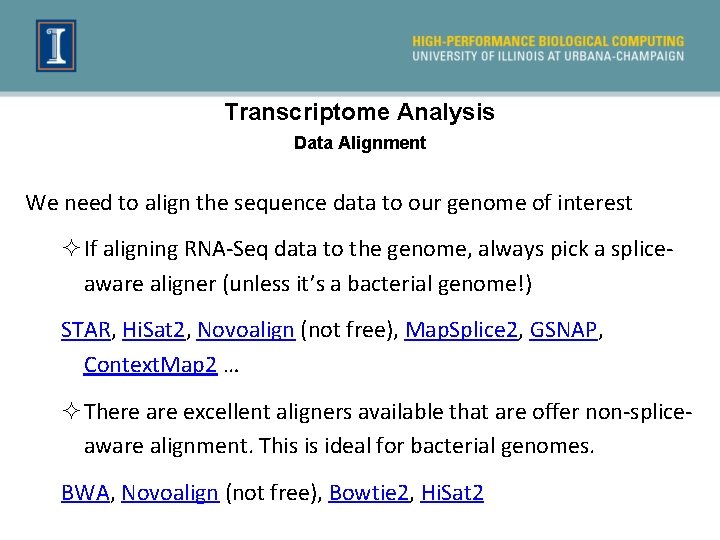
Transcriptome Analysis Data Alignment We need to align the sequence data to our genome of interest ²If aligning RNA-Seq data to the genome, always pick a spliceaware aligner (unless it’s a bacterial genome!) STAR, Hi. Sat 2, Novoalign (not free), Map. Splice 2, GSNAP, Context. Map 2 … ²There are excellent aligners available that are offer non-spliceaware alignment. This is ideal for bacterial genomes. BWA, Novoalign (not free), Bowtie 2, Hi. Sat 2

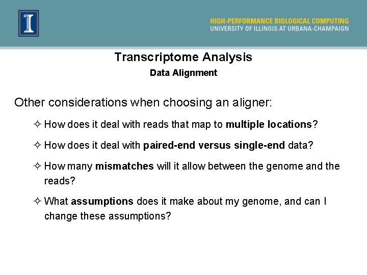
Transcriptome Analysis Data Alignment Other considerations when choosing an aligner: ² How does it deal with reads that map to multiple locations? ² How does it deal with paired-end versus single-end data? ² How many mismatches will it allow between the genome and the reads? ² What assumptions does it make about my genome, and can I change these assumptions?

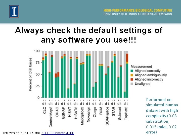
Always check the default settings of any software you use!!! Baruzzo et. al, 2017, doi: 10. 1038/nmeth. 4106 Performed on simulated human dataset with high complexity (0. 03 substitution, 0. 005 indel, 0. 02 error)

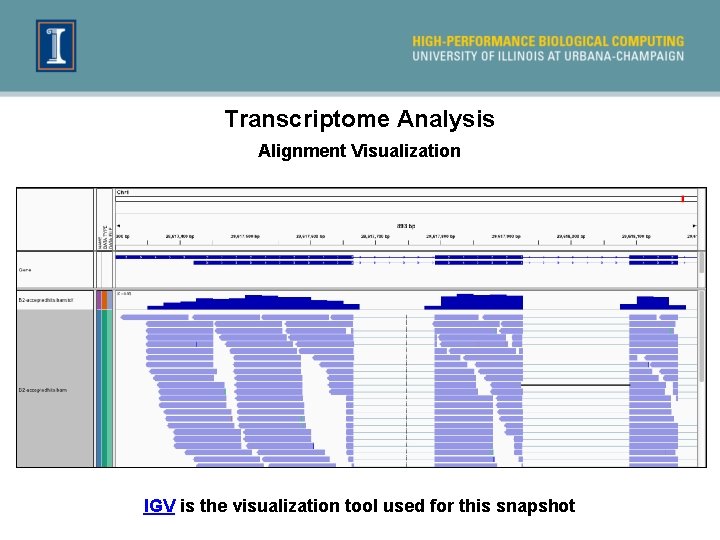
Transcriptome Analysis Alignment Visualization IGV is the visualization tool used for this snapshot

General Outline 4. Transcriptomic analysis methods and tools a. Transcriptome Analysis; aspects common to both assembly and differential gene expression ² Download data ² Quality check ² Data alignment b. Assembly c. Differential Gene Expression d. Choosing a method, the considerations… e. Final thoughts and observations

Transcriptome Assembly Overview Two main types of assembly a. Reference-based assembly b. A de novo assembly

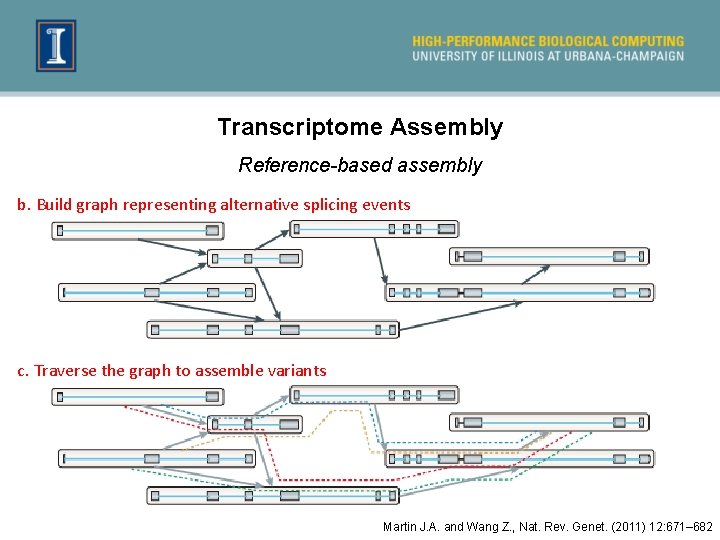
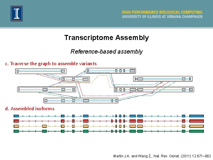
Transcriptome Assembly Reference-based assembly Used when the genome reference sequence is known, and: ² Transcriptome data is not available ² Transcriptome data is available but not good enough, ² i. e. missing isoforms of genes, or unknown non-coding regions ² The existing transcriptome information is for a different tissue type ² Stringtie, and Scripture are some reference-based transcriptome assemblers

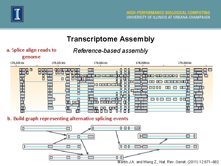
Transcriptome Assembly a. Splice align reads to genome Reference-based assembly b. Build graph representing alternative splicing events Martin J. A. and Wang Z. , Nat. Rev. Genet. (2011) 12: 671– 682

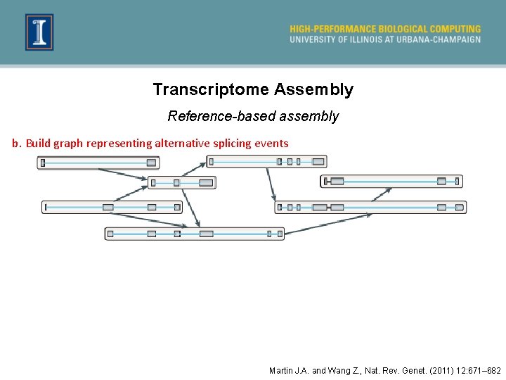
Transcriptome Assembly Reference-based assembly b. Build graph representing alternative splicing events Martin J. A. and Wang Z. , Nat. Rev. Genet. (2011) 12: 671– 682

Transcriptome Assembly Reference-based assembly b. Build graph representing alternative splicing events c. Traverse the graph to assemble variants Martin J. A. and Wang Z. , Nat. Rev. Genet. (2011) 12: 671– 682

Transcriptome Assembly Reference-based assembly c. Traverse the graph to assemble variants d. Assembled isoforms Martin J. A. and Wang Z. , Nat. Rev. Genet. (2011) 12: 671– 682

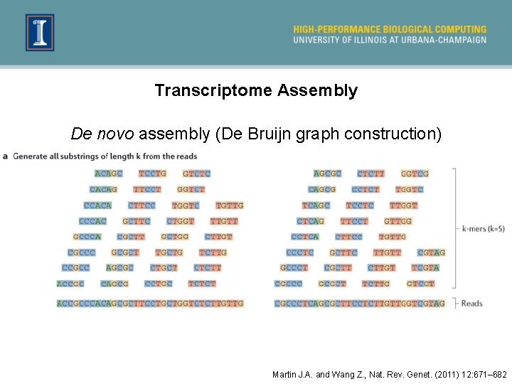
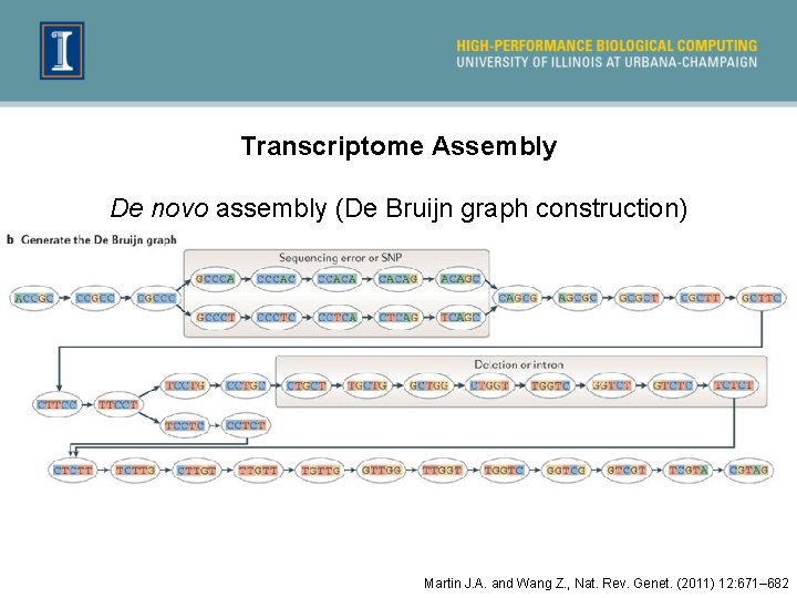
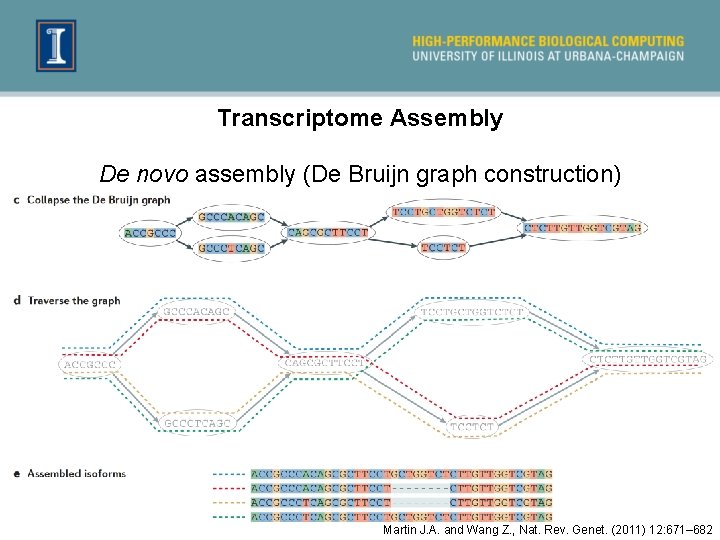
Transcriptome Assembly De novo assembly Used when very little information is available for the genome ² Often the first step in putting together information about an unknown genome ² Amount of data needed for a good de novo assembly is higher than what is needed for a reference-based assembly ² Can be used for genome annotation, once the genome is assembled ² Trinity, SPAdes, and Trans. ABy. SS, are examples of well-regarded transcriptome assemblers

Transcriptome Assembly De novo assembly (De Bruijn graph construction) Martin J. A. and Wang Z. , Nat. Rev. Genet. (2011) 12: 671– 682

Transcriptome Assembly De novo assembly (De Bruijn graph construction) Martin J. A. and Wang Z. , Nat. Rev. Genet. (2011) 12: 671– 682

Transcriptome Assembly De novo assembly (De Bruijn graph construction) Martin J. A. and Wang Z. , Nat. Rev. Genet. (2011) 12: 671– 682

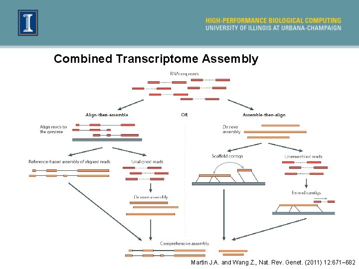
Combined Transcriptome Assembly Martin J. A. and Wang Z. , Nat. Rev. Genet. (2011) 12: 671– 682

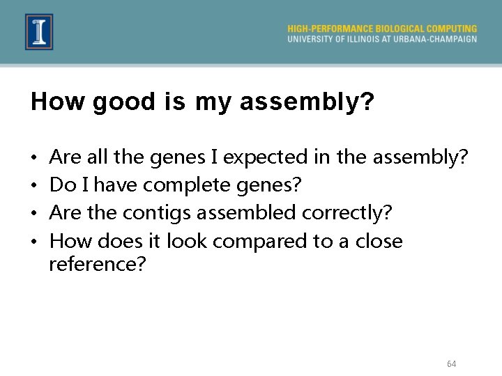
How good is my assembly? • • Are all the genes I expected in the assembly? Do I have complete genes? Are the contigs assembled correctly? How does it look compared to a close reference? 64

Tools for Evaluating Assembly: using the information you have Trans. Rate – evaluates assembly using reads, paired end information, reference genome, protein data, etc. • Can generate a ‘cleaned-up’ or optimized assembly based on metrics DETONATE – evaluates assembly based on read mapping and/or reference information

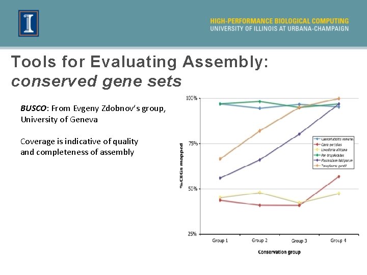
Tools for Evaluating Assembly: conserved gene sets BUSCO: From Evgeny Zdobnov’s group, University of Geneva Coverage is indicative of quality and completeness of assembly

Outline 3. Transcriptomic analysis methods and tools a. Transcriptome Analysis; aspects common to both assembly and differential gene expression ² Quality check ² Data alignment b. Assembly c. Differential Gene Expression d. Choosing a method, the considerations… e. Final thoughts and observations

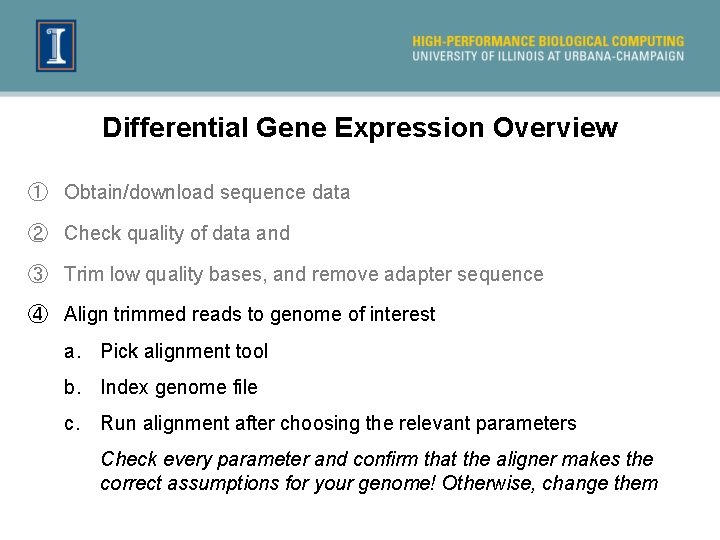
Differential Gene Expression Overview ① Obtain/download sequence data ② Check quality of data and ③ Trim low quality bases, and remove adapter sequence ④ Align trimmed reads to genome of interest a. Pick alignment tool b. Index genome file c. Run alignment after choosing the relevant parameters Check every parameter and confirm that the aligner makes the correct assumptions for your genome! Otherwise, change them

Differential Gene Expression overview ④ Set up to do differential gene expression (DGE) Identify read counts associated with genes a. Do you want to obtain raw read counts or normalized read counts? This will depend on the statistical analysis you wish to perform downstream ² htseq & feature-counts return raw read counts ² Required for R programs like DESeq & Edge. R ² String. Tie returns FPKM normalized counts for each gene

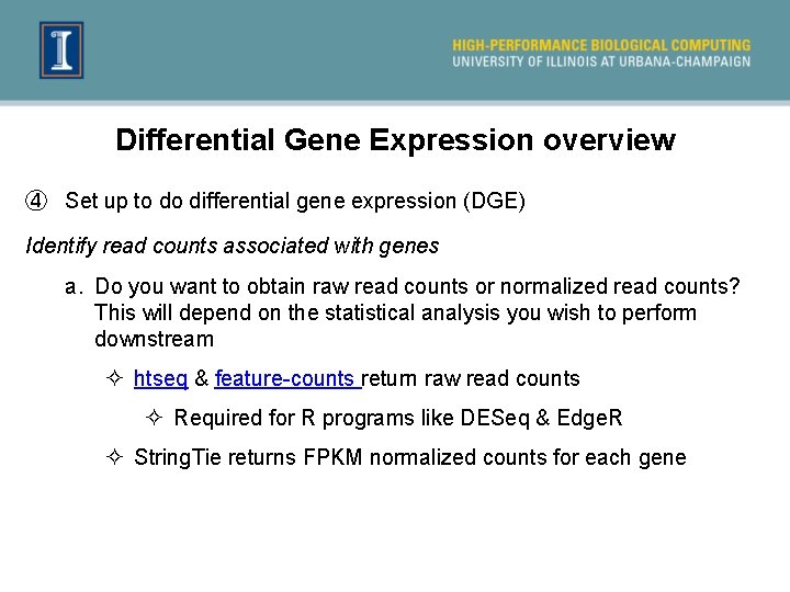
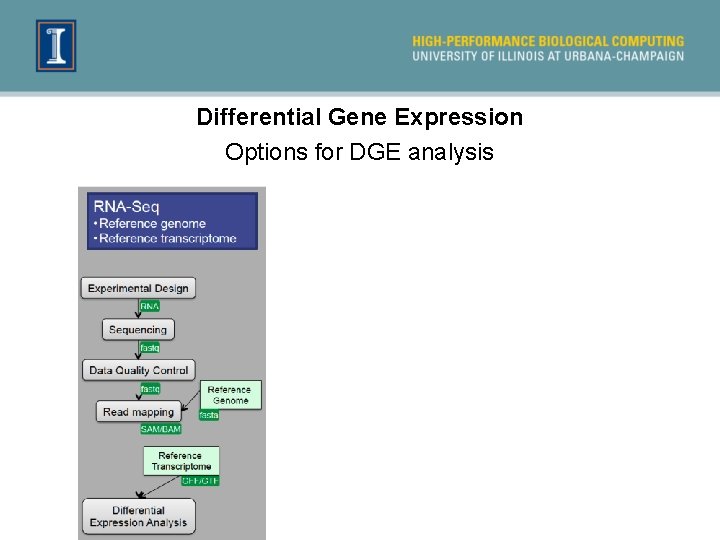
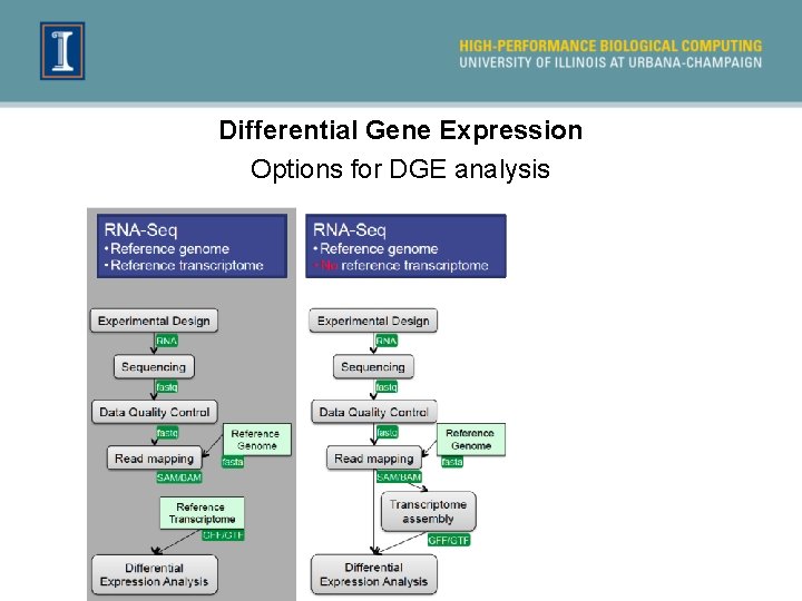
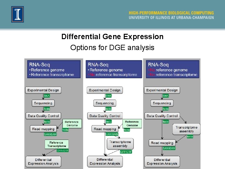
Differential Gene Expression Options for DGE analysis

Differential Gene Expression Options for DGE analysis

Differential Gene Expression Options for DGE analysis

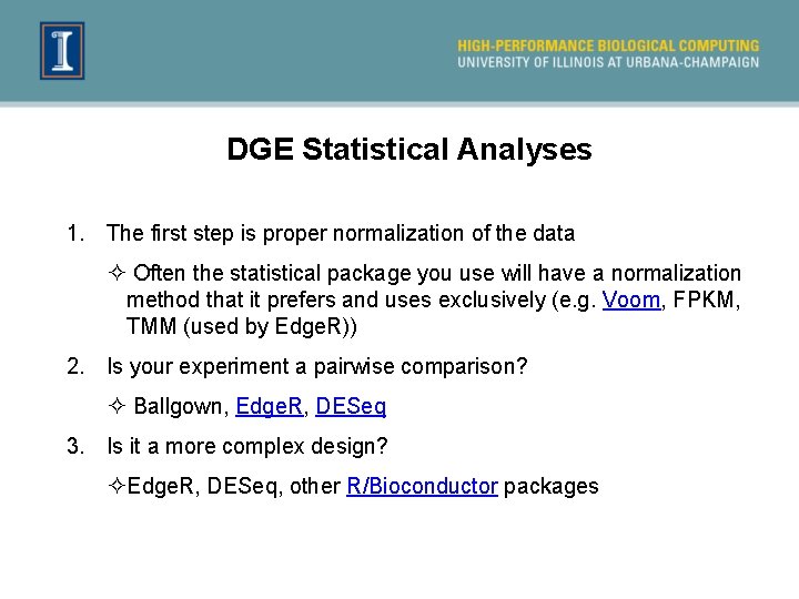
DGE Statistical Analyses 1. The first step is proper normalization of the data ² Often the statistical package you use will have a normalization method that it prefers and uses exclusively (e. g. Voom, FPKM, TMM (used by Edge. R)) 2. Is your experiment a pairwise comparison? ² Ballgown, Edge. R, DESeq 3. Is it a more complex design? ²Edge. R, DESeq, other R/Bioconductor packages

Statistical Results • A list of significantly differentially expressed genes • Heatmaps, Venn Diagrams, and more • Annotation • WGCNA • . . . and more!

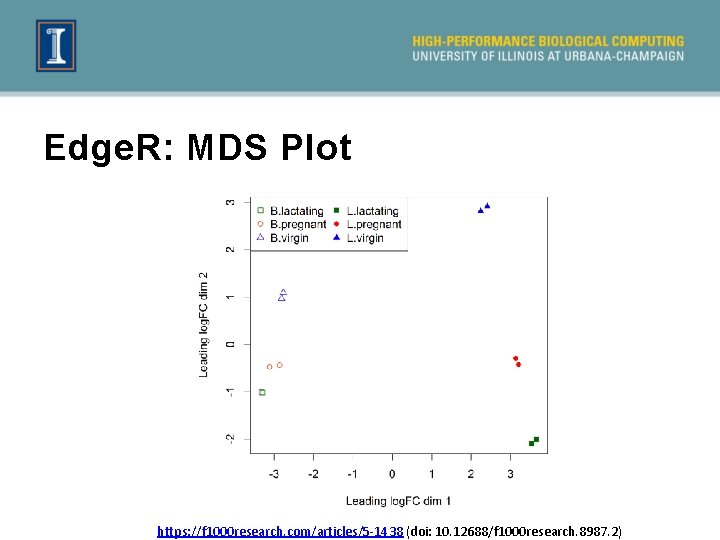
Edge. R: MDS Plot https: //f 1000 research. com/articles/5 -1438 (doi: 10. 12688/f 1000 research. 8987. 2)

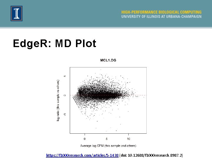
Edge. R: MD Plot https: //f 1000 research. com/articles/5 -1438 (doi: 10. 12688/f 1000 research. 8987. 2)

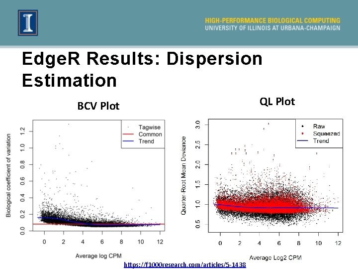
Edge. R Results: Dispersion Estimation QL Plot BCV Plot https: //f 1000 research. com/articles/5 -1438

TRANSCRIPT COUNTING METHODS

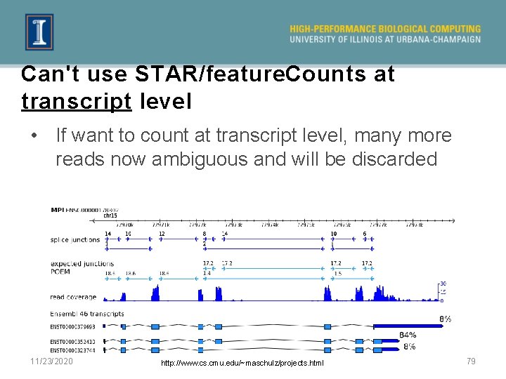
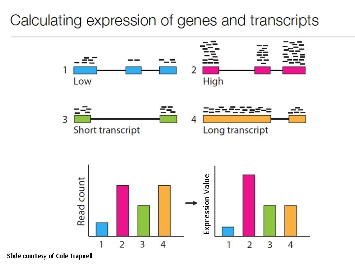
Can't use STAR/feature. Counts at transcript level • If want to count at transcript level, many more reads now ambiguous and will be discarded 11/23/2020 http: //www. cs. cmu. edu/~maschulz/projects. html 79

Problems with STAR/feature. Counts at gene level: 1. Multimapping reads not used, leading to underestimation of gene abundances, particularly for genes with more shared sequence 2. A small percentage of genes may not ever be quantifiable using this method. 3. Genes that change relative isoform usage can have erroneous results due to changes in 11/23/2020 80 isoform length

Expression Value Slide courtesy of Cole Trapnell

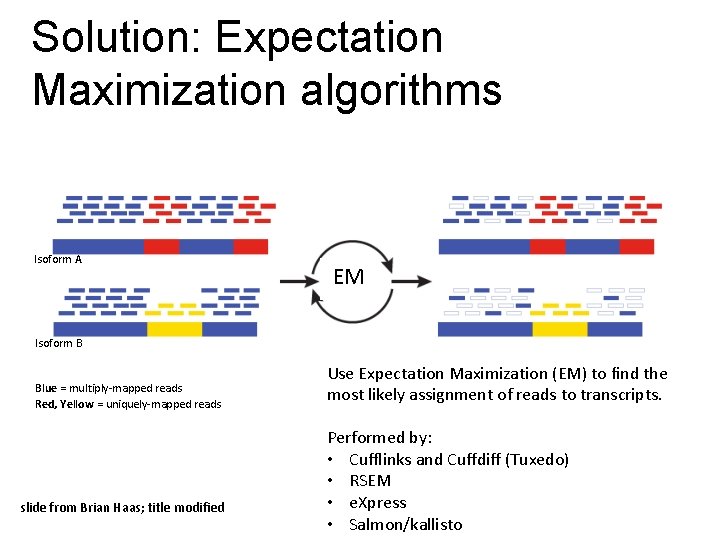
Solution: Expectation Maximization algorithms Isoform A EM Isoform B Blue = multiply-mapped reads Red, Yellow = uniquely-mapped reads slide from Brian Haas; title modified Use Expectation Maximization (EM) to find the most likely assignment of reads to transcripts. Performed by: • Cufflinks and Cuffdiff (Tuxedo) • RSEM • e. Xpress • Salmon/kallisto

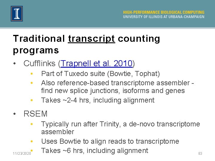
Traditional transcript counting programs • Cufflinks (Trapnell et al. 2010) • • • Part of Tuxedo suite (Bowtie, Tophat) Also reference-based transcriptome assembler - find new splice junctions, isoforms and genes Takes ~2 -4 hrs, including alignment • RSEM • • • 11/23/2020 Typically run after Trinity, a de-novo transcriptome assembler Uses Bowtie to align reads to transcriptome Takes ~6 hrs, including alignment 83

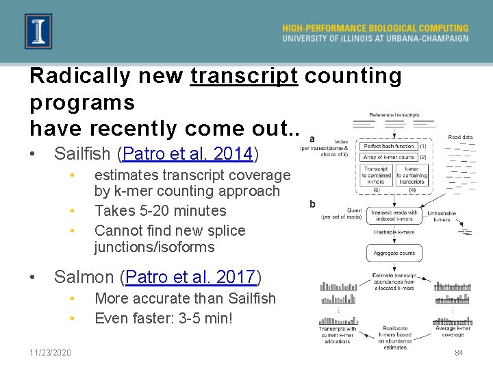
Radically new transcript counting programs have recently come out. . . • Sailfish (Patro et al. 2014) • • estimates transcript coverage by k-mer counting approach Takes 5 -20 minutes Cannot find new splice junctions/isoforms Salmon (Patro et al. 2017) • • 11/23/2020 More accurate than Sailfish Even faster: 3 -5 min! 84

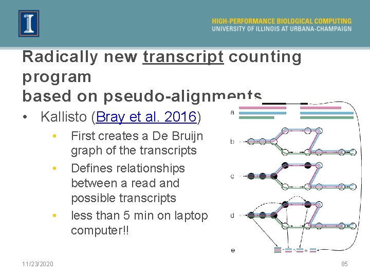
Radically new transcript counting program based on pseudo-alignments • Kallisto (Bray et al. 2016) • • • 11/23/2020 First creates a De Bruijn graph of the transcripts Defines relationships between a read and possible transcripts less than 5 min on laptop computer!! 85

When to use transcript-counting methods • Genome duplications • Many gene families • When you have a large percentage (>15%) of multi-mapped reads Note: After counting at the transcript-level, you can then group by gene-level, which is more accurate.

Outline 3. Transcriptomic analysis methods and tools a. Transcriptome Analysis; aspects common to both assembly and differential gene expression ² Download data ² Quality check ² Data alignment b. Assembly c. Differential Gene Expression d. Choosing a method, the considerations… e. Final thoughts and observations

Transcriptome Analysis How does one pick the right tools?

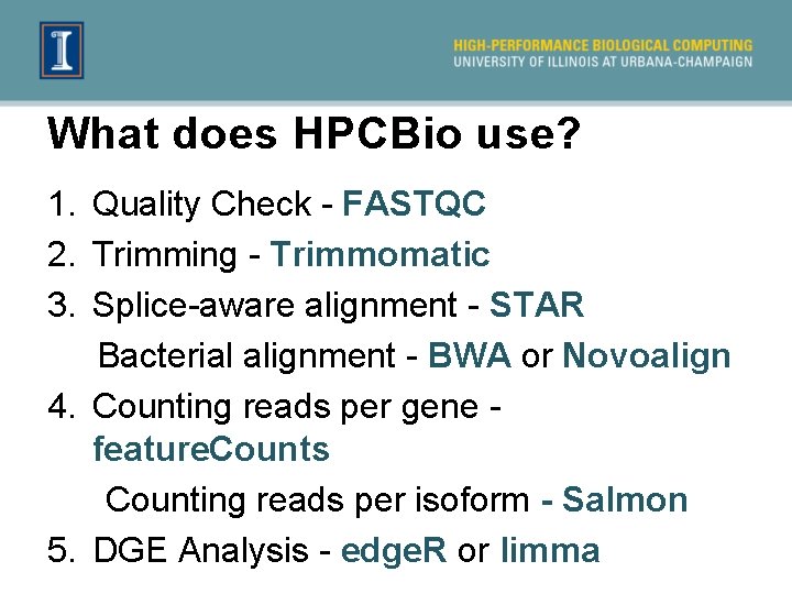
What does HPCBio use? 1. Quality Check - FASTQC 2. Trimming - Trimmomatic 3. Splice-aware alignment - STAR Bacterial alignment - BWA or Novoalign 4. Counting reads per gene - feature. Counts Counting reads per isoform - Salmon 5. DGE Analysis - edge. R or limma

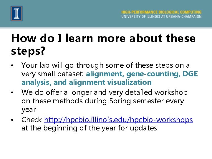
How do I learn more about these steps? • • • Your lab will go through some of these steps on a very small dataset: alignment, gene-counting, DGE analysis, and alignment visualization We do offer a longer and very detailed workshop on these methods during Spring semester every year Check http: //hpcbio. illinois. edu/hpcbio-workshops at the beginning of the year for updates

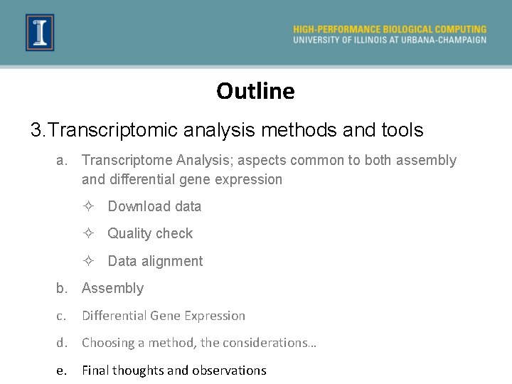
Outline 3. Transcriptomic analysis methods and tools a. Transcriptome Analysis; aspects common to both assembly and differential gene expression ² Download data ² Quality check ² Data alignment b. Assembly c. Differential Gene Expression d. Choosing a method, the considerations… e. Final thoughts and observations

Final thoughts and stray observations 1. Think carefully about what your experimental goals are before designing your experiment and choosing your bioinformatics tools

Final thoughts and stray observations 1. Think carefully about what your experimental goals are before designing your experiment and choosing your bioinformatics tools 2. When in doubt “Google it” and ask questions. http: //www. biostars. org/ - Biostar (Bioinformatics explained) http: //seqanswers. com/ - SEQanswers (the next generation sequencing community)

Final thoughts and stray observations 1. Think carefully about what your experimental goals are before designing your experiment and choosing your bioinformatics tools 2. When in doubt “Google it” and ask questions. http: //www. biostars. org/ - Biostar (Bioinformatics explained) http: //seqanswers. com/ - SEQanswers (the next generation sequencing community) 3. Another good resource if you are not ready to use the command line routinely is Galaxy. It is a web-based bioinformatics portal that can be locally installed, if you have the necessary computational infrastructure.

Final thoughts and stray observations 4. Today we covered how to deal with Illumina data, but you may also encounter long-read data as well • Hybrid transcriptome assemblies can be done, but are usually challenging

Final thoughts and stray observations 4. Today we covered how to deal with Illumina data, but you may also encounter long-read data as well • Hybrid assemblies can be done, but are usually challenging 5. R is an excellent language to learn, if you are interested in performing indepth statistical analyses for differential gene expression analysis • Not within the scope of this lecture/lab section • We do offer a long RNA-Seq workshop that covers the “HPCBio” RNASeq pipeline: http: //hpcbio. illinois. edu/hpcbio-workshops

Documentation and Support Online resources for RNA-Seq analysis questions – ²Software manuals ²http: //www. biostars. org/ - Biostar (Bioinformatics explained) ²http: //seqanswers. com/ - SEQanswers (the next generation sequencing community) ²Most tools have a dedicated lists/forums Contact us at: hpcbiohelp@illinois. edu hpcbiotraining@igb. illinois. edu jholmes 5@illinois. edu See website for upcoming workshops & services: http: //hpcbio. illinois. edu/

Thank you for your attention!