Introduction to RNASeq Transcriptome Analysis Jessica Holmes Power

Introduction to RNA-Seq & Transcriptome Analysis Jessica Holmes Power. Point by Shayan Tabe Bordbar Edited by Negin Valizadegan 2021 RNA-Seq Lab | 2020 1

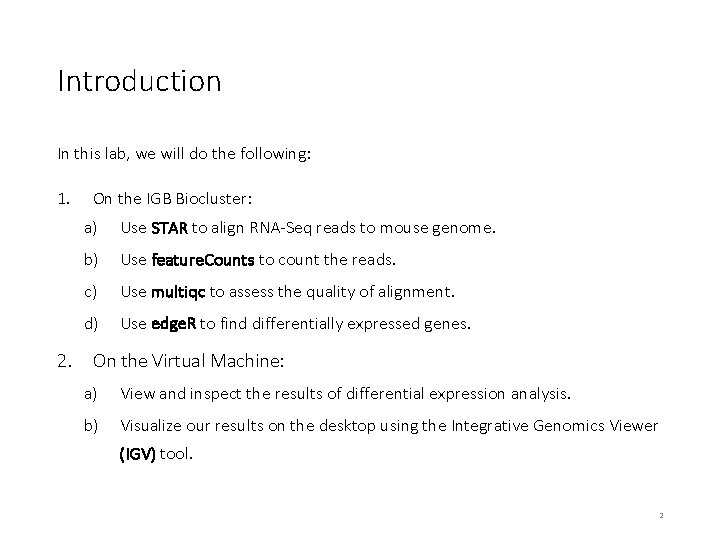
Introduction In this lab, we will do the following: 1. 2. On the IGB Biocluster: a) Use STAR to align RNA-Seq reads to mouse genome. b) Use feature. Counts to count the reads. c) Use multiqc to assess the quality of alignment. d) Use edge. R to find differentially expressed genes. On the Virtual Machine: a) View and inspect the results of differential expression analysis. b) Visualize our results on the desktop using the Integrative Genomics Viewer (IGV) tool. 2

Start the VM • Follow instructions for starting VM. (This is the Remote Desktop software. ) • The instructions are different for UIUC and Mayo participants. • Find the instructions for this on the course website under Lab Set-up: https: //publish. illinois. edu/compgenomicscourse/2021 -schedule/ Variant Calling Workshop | Chris Fields | 2020 3

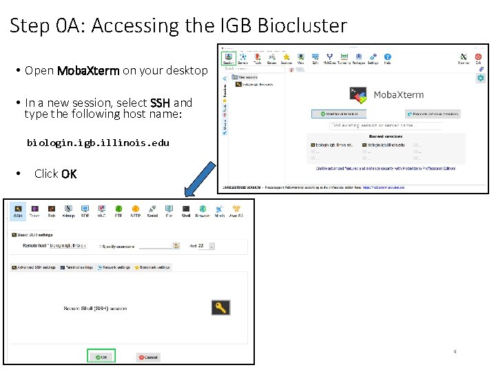
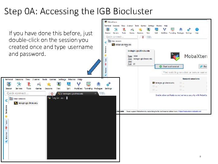
Step 0 A: Accessing the IGB Biocluster • Open Moba. Xterm on your desktop • In a new session, select SSH and type the following host name: biologin. igb. illinois. edu • Click OK 4

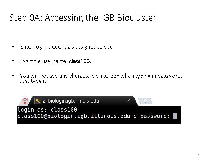
Step 0 A: Accessing the IGB Biocluster • Enter login credentials assigned to you. • Example username: class 100. • You will not see any characters on screen when typing in password. Just type it. 5

Step 0 A: Accessing the IGB Biocluster If you have done this before, just double-click on the session you created once and type username and password. 6

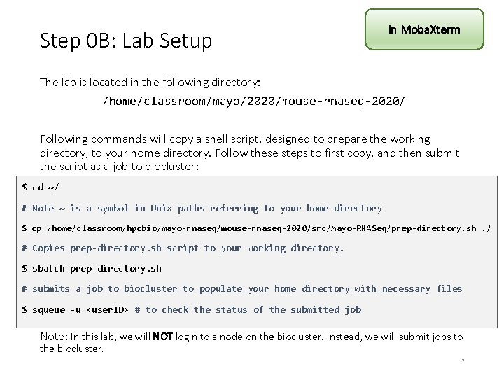
Step 0 B: Lab Setup In Moba. Xterm The lab is located in the following directory: /home/classroom/mayo/2020/mouse-rnaseq-2020/ Following commands will copy a shell script, designed to prepare the working directory, to your home directory. Follow these steps to first copy, and then submit the script as a job to biocluster: $ cd ~/ # Note ~ is a symbol in Unix paths referring to your home directory $ cp /home/classroom/hpcbio/mayo-rnaseq/mouse-rnaseq-2020/src/Mayo-RNASeq/prep-directory. sh. / # Copies prep-directory. sh script to your working directory. $ sbatch prep-directory. sh # submits a job to biocluster to populate your home directory with necessary files $ squeue -u <user. ID> # to check the status of the submitted job Note: In this lab, we will NOT login to a node on the biocluster. Instead, we will submit jobs to the biocluster. 7

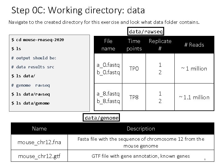
Step 0 C: Working directory: data Navigate to the created directory for this exercise and look what data folder contains. data/rawseq $ cd mouse-rnaseq-2020 $ ls File name Time points Replicate # # Reads a_0. fastq b_0. fastq TP 0 1 2 ~ 1 million a_8. fastq b_8. fastq TP 8 1 2 ~ 1. 1 million # output should be: # data results src $ ls data/ # genome rawseq $ ls data/genome Name Description mouse_chr 12. fna Fasta file with the sequence of chromosome 12 from the mouse genome mouse_chr 12. gtf GTF file with gene annotation, known genes 8

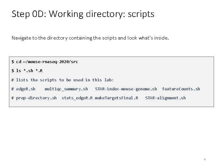
Step 0 D: Working directory: scripts Navigate to the directory containing the scripts and look what’s inside. $ cd ~/mouse-rnaseq-2020/src $ ls *. sh *. R # lists the scripts to be used in this lab: # edge. R. sh multiqc_summary. sh # prep-directory. sh STAR-index-mouse-genome. sh stats_edge. R. R make. Targets. Final. R feature. Counts. sh STAR-alignment. sh 9

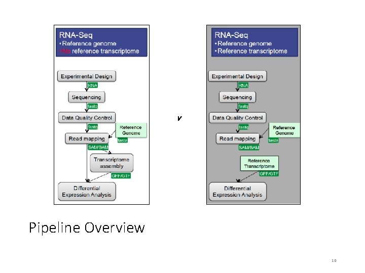
v Pipeline Overview 10

Step 1: Alignment using STAR In this exercise, we will be aligning RNA-Seq reads to a reference genome. 11

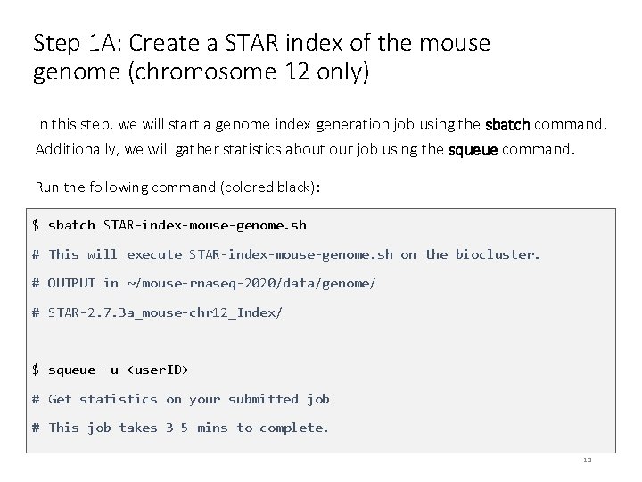
Step 1 A: Create a STAR index of the mouse genome (chromosome 12 only) In this step, we will start a genome index generation job using the sbatch command. Additionally, we will gather statistics about our job using the squeue command. Run the following command (colored black): $ sbatch STAR-index-mouse-genome. sh # This will execute STAR-index-mouse-genome. sh on the biocluster. # OUTPUT in ~/mouse-rnaseq-2020/data/genome/ # STAR-2. 7. 3 a_mouse-chr 12_Index/ $ squeue –u <user. ID> # Get statistics on your submitted job # This job takes 3 -5 mins to complete. 12

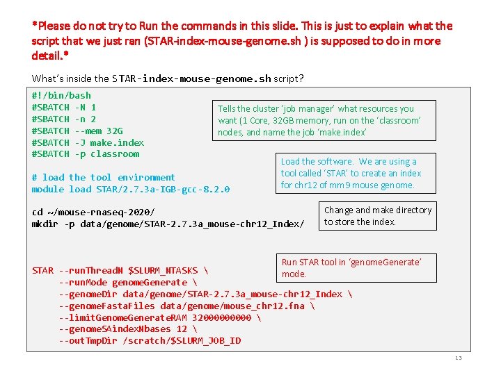
*Please do not try to Run the commands in this slide. This is just to explain what the script that we just ran (STAR-index-mouse-genome. sh ) is supposed to do in more detail. * What’s inside the STAR-index-mouse-genome. sh script? #!/bin/bash #SBATCH -N 1 #SBATCH -n 2 #SBATCH --mem 32 G #SBATCH -J make. index #SBATCH -p classroom Tells the cluster ‘job manager’ what resources you want (1 Core, 32 GB memory, run on the ‘classroom’ nodes, and name the job ‘make. index’ # load the tool environment module load STAR/2. 7. 3 a-IGB-gcc-8. 2. 0 Load the software. We are using a tool called ‘STAR’ to create an index for chr 12 of mm 9 mouse genome. cd ~/mouse-rnaseq-2020/ mkdir -p data/genome/STAR-2. 7. 3 a_mouse-chr 12_Index/ Change and make directory to store the index. Run STAR tool in ‘genome. Generate’ STAR --run. Thread. N $SLURM_NTASKS mode. --run. Mode genome. Generate --genome. Dir data/genome/STAR-2. 7. 3 a_mouse-chr 12_Index --genome. Fasta. Files data/genome/mouse_chr 12. fna --limit. Genome. Generate. RAM 3200000 --genome. SAindex. Nbases 12 --out. Tmp. Dir /scratch/$SLURM_JOB_ID 13

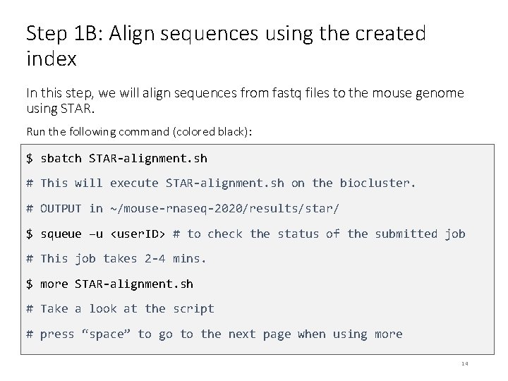
Step 1 B: Align sequences using the created index In this step, we will align sequences from fastq files to the mouse genome using STAR. Run the following command (colored black): $ sbatch STAR-alignment. sh # This will execute STAR-alignment. sh on the biocluster. # OUTPUT in ~/mouse-rnaseq-2020/results/star/ $ squeue –u <user. ID> # to check the status of the submitted job # This job takes 2 -4 mins. $ more STAR-alignment. sh # Take a look at the script # press “space” to go to the next page when using more 14

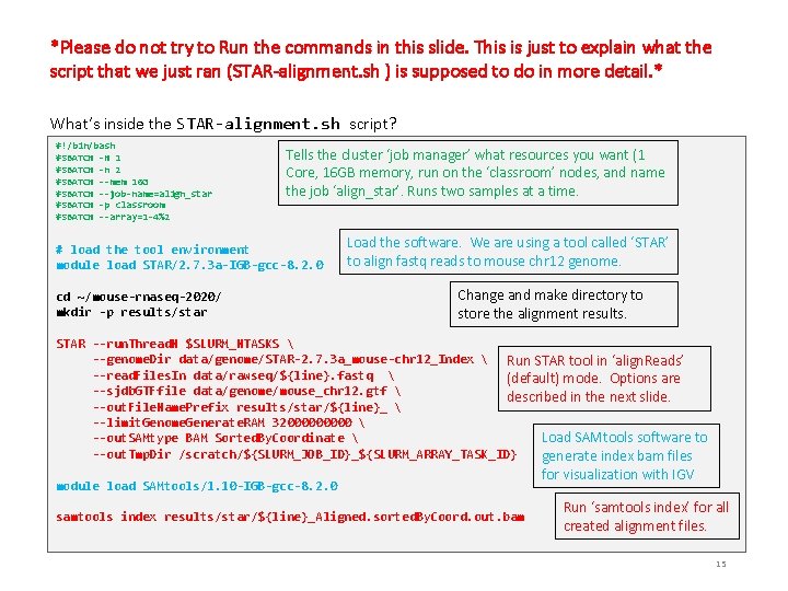
*Please do not try to Run the commands in this slide. This is just to explain what the script that we just ran (STAR-alignment. sh ) is supposed to do in more detail. * What’s inside the STAR-alignment. sh script? #!/bin/bash #SBATCH -N 1 #SBATCH -n 2 #SBATCH --mem 16 G #SBATCH --job-name=align_star #SBATCH -p classroom #SBATCH --array=1 -4%2 Tells the cluster ‘job manager’ what resources you want (1 Core, 16 GB memory, run on the ‘classroom’ nodes, and name the job ‘align_star’. Runs two samples at a time. # load the tool environment module load STAR/2. 7. 3 a-IGB-gcc-8. 2. 0 cd ~/mouse-rnaseq-2020/ mkdir -p results/star Load the software. We are using a tool called ‘STAR’ to align fastq reads to mouse chr 12 genome. Change and make directory to store the alignment results. STAR --run. Thread. N $SLURM_NTASKS --genome. Dir data/genome/STAR-2. 7. 3 a_mouse-chr 12_Index Run STAR tool in ‘align. Reads’ --read. Files. In data/rawseq/${line}. fastq (default) mode. Options are --sjdb. GTFfile data/genome/mouse_chr 12. gtf described in the next slide. --out. File. Name. Prefix results/star/${line}_ --limit. Genome. Generate. RAM 3200000 Load SAMtools software to --out. SAMtype BAM Sorted. By. Coordinate --out. Tmp. Dir /scratch/${SLURM_JOB_ID}_${SLURM_ARRAY_TASK_ID} generate index bam files module load SAMtools/1. 10 -IGB-gcc-8. 2. 0 samtools index results/star/${line}_Aligned. sorted. By. Coord. out. bam for visualization with IGV Run ‘samtools index’ for all created alignment files. 15

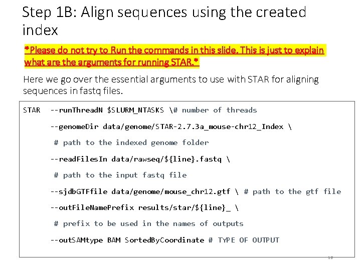
Step 1 B: Align sequences using the created index *Please do not try to Run the commands in this slide. This is just to explain what are the arguments for running STAR. * Here we go over the essential arguments to use with STAR for aligning sequences in fastq files. STAR --run. Thread. N $SLURM_NTASKS # number of threads --genome. Dir data/genome/STAR-2. 7. 3 a_mouse-chr 12_Index # path to the indexed genome folder --read. Files. In data/rawseq/${line}. fastq # path to the input fastq file --sjdb. GTFfile data/genome/mouse_chr 12. gtf # path to the gtf file --out. File. Name. Prefix results/star/${line}_ # prefix to be used in the names of outputs --out. SAMtype BAM Sorted. By. Coordinate # TYPE OF OUTPUT 16

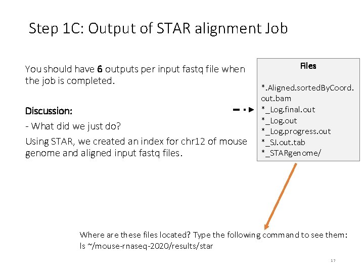
Step 1 C: Output of STAR alignment Job You should have 6 outputs per input fastq file when the job is completed. Discussion: - What did we just do? Using STAR, we created an index for chr 12 of mouse genome and aligned input fastq files. Files *. Aligned. sorted. By. Coord. out. bam *_Log. final. out *_Log. progress. out *_SJ. out. tab *_STARgenome/ Where are these files located? Type the following command to see them: ls ~/mouse-rnaseq-2020/results/star 17

Step 2: Read aligned counts Use feature. Counts to generate the aligned counts for each of the bam files generated in step 1. 18

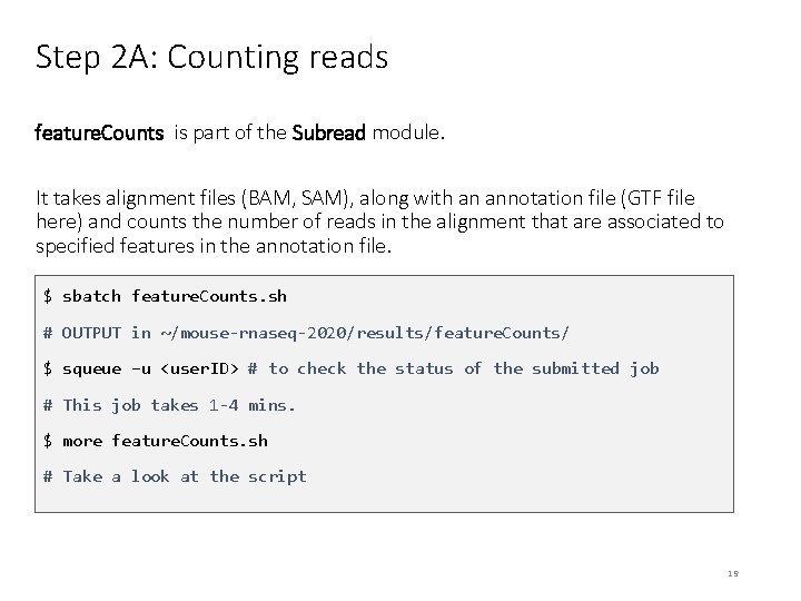
Step 2 A: Counting reads feature. Counts is part of the Subread module. It takes alignment files (BAM, SAM), along with an annotation file (GTF file here) and counts the number of reads in the alignment that are associated to specified features in the annotation file. $ sbatch feature. Counts. sh # OUTPUT in ~/mouse-rnaseq-2020/results/feature. Counts/ $ squeue –u <user. ID> # to check the status of the submitted job # This job takes 1 -4 mins. $ more feature. Counts. sh # Take a look at the script 19

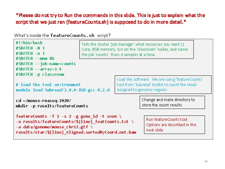
*Please do not try to Run the commands in this slide. This is just to explain what the script that we just ran (feature. Counts. sh) is supposed to do in more detail. * What’s inside the feature. Counts. sh script? #!/bin/bash #SBATCH -N 1 #SBATCH -n 1 #SBATCH --mem 8 G #SBATCH --job-name=counts #SBATCH --array=1 -4 #SBATCH -p classroom Tells the cluster ‘job manager’ what resources you want (1 Core, 8 GB memory, run on the ‘classroom’ nodes, and name the job ‘counts’. Runs 4 samples at a time. # load the tool environment module load Subread/2. 0. 0 -IGB-gcc-8. 2. 0 Load the software. We are using ‘feature. Counts’ tool from ‘Subread’ toolkit to count the reads assigned to genomic regions. cd ~/mouse-rnaseq-2020/ mkdir -p results/feature. Counts -T 1 -s 2 -g gene_id -t exon -o results/feature. Counts/${line}_feat. Counts. txt -a data/genome/mouse_chr 12. gtf results/star/${line}_Aligned. sorted. By. Coord. out. bam Change and make directory to store the count results. Run feature. Counts tool. Options are described in the next slide. 20

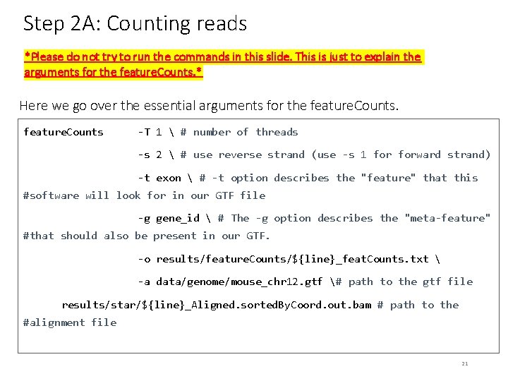
Step 2 A: Counting reads *Please do not try to run the commands in this slide. This is just to explain the arguments for the feature. Counts. * Here we go over the essential arguments for the feature. Counts -T 1 # number of threads -s 2 # use reverse strand (use -s 1 forward strand) -t exon # -t option describes the "feature" that this #software will look for in our GTF file -g gene_id # The -g option describes the "meta-feature" #that should also be present in our GTF. -o results/feature. Counts/${line}_feat. Counts. txt -a data/genome/mouse_chr 12. gtf # path to the gtf file results/star/${line}_Aligned. sorted. By. Coord. out. bam # path to the #alignment file 21

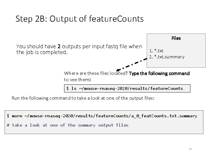
Step 2 B: Output of feature. Counts Files You should have 2 outputs per input fastq file when the job is completed. 1. *. txt 2. *. txt. summary Where are these files located? Type the following command to see them: $ ls ~/mouse-rnaseq-2020/results/feature. Counts Run the following command to take a look at one of the output files: $ more ~/mouse-rnaseq-2020/results/feature. Counts/a_0_feat. Counts. txt. summary # take a look at one of the summary output files 22

Step 3: Using Multi. QC to generate quality report Now we will use Multi. QC to assess the quality of alignments and to collate STAR and feature. Counts numbers. We will also use a R script to generate plots on read mappings. 23

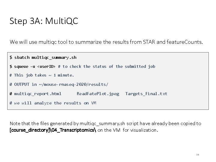
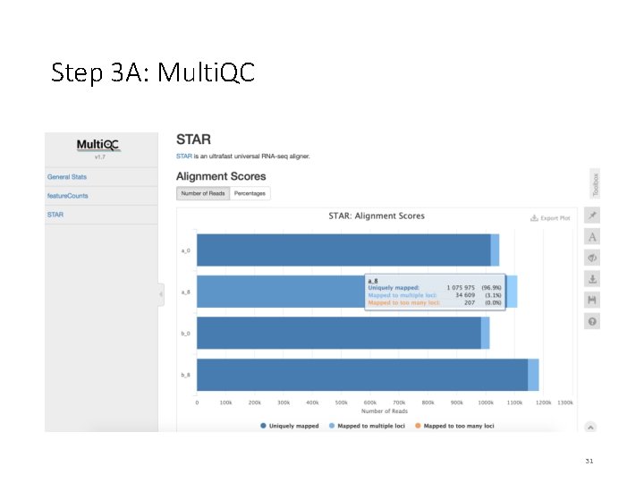
Step 3 A: Multi. QC We will use multiqc tool to summarize the results from STAR and feature. Counts. $ sbatch multiqc_summary. sh $ squeue –u <user. ID> # to check the status of the submitted job # This job takes ~ 1 minute. # OUTPUT in ~/mouse-rnaseq-2020/results/ # multiqc_report. html Read. Fate. Plot. jpeg Targets_Final. txt # we will analyze the results on VM Note that the files generated by multiqc_summary. sh script have already been copied to [course_directory]4_Transcriptomics on the VM for visualization. 24

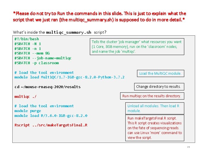
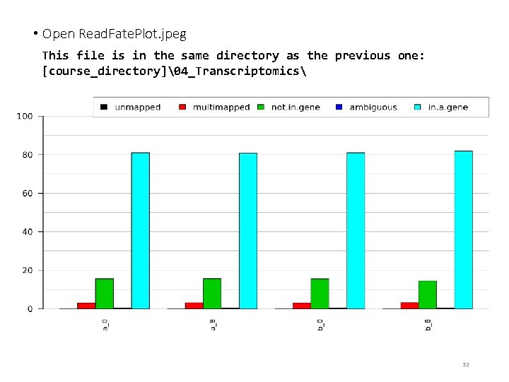
*Please do not try to Run the commands in this slide. This is just to explain what the script that we just ran (the multiqc_summary. sh) is supposed to do in more detail. * What’s inside the multiqc_summary. sh script? #!/bin/bash #SBATCH -N 1 #SBATCH -n 1 #SBATCH --mem 8 G #SBATCH --job-name=multiqc #SBATCH -p classroom Tells the cluster ‘job manager’ what resources you want (1 Core, 8 GB memory), run on the ‘classroom’ nodes, and name the job ‘multiqc’. # load the tool environment module load Multi. QC/1. 7 -IGB-gcc-8. 2. 0 -Python-3. 7. 2 cd ~/mouse-rnaseq-2020/results multiqc. / # load the tool environment module purge module load R/3. 6. 0 -IGB-gcc-8. 2. 0 Rscript. . /src/make. Targets. Final. R Load the Multi. QC module. Change directory to results. Run multiqc on the results directory. Unload all modules. Then load R module. Run make. Targets. Final. R script. This R script creates visualizations on the fate of sequencing reads. can use Linux ‘more’ command to view the script. 25

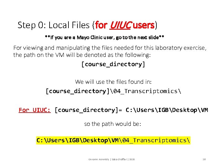
Step 0: Local Files (for UIUC users) **If you are a Mayo Clinic user, go to the next slide** For viewing and manipulating the files needed for this laboratory exercise, the path on the VM will be denoted as the following: [course_directory] We will use the files found in: [course_directory]4_Transcriptomics For UIUC: [course_directory]= C: UsersIGBDesktopVM so the path would be: C: UsersIGBDesktopVM4_Transcriptomics Genome Assembly | Saba Ghaffari | 2020 26

Step 0: Local Files (for Mayo Clinic users) For viewing and manipulating the files needed for this laboratory exercise, the path on the VM will be denoted as the following: [course_directory] We will use the files found in: [course_directory]4_Transcriptomics For Mayo Clinic: [course_directory]= C: /Users/Public/Desktop/VM so the path would be: C: UsersPublicDesktopVM4_Transcriptomics Genome Assembly | Saba Ghaffari | 2020 27

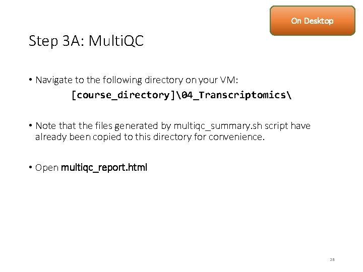
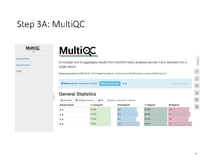
On Desktop Step 3 A: Multi. QC • Navigate to the following directory on your VM: [course_directory]4_Transcriptomics • Note that the files generated by multiqc_summary. sh script have already been copied to this directory for convenience. • Open multiqc_report. html 28

Step 3 A: Multi. QC 29

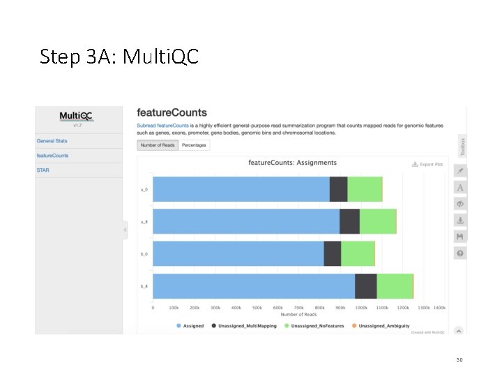
Step 3 A: Multi. QC 30

Step 3 A: Multi. QC 31

• Open Read. Fate. Plot. jpeg This file is in the same directory as the previous one: [course_directory]4_Transcriptomics 32

Step 4: Finding differentially expressed genes Now we will use edge. R to analyze the count files generated in step 2 to find differentially expressed genes between two time points. 33

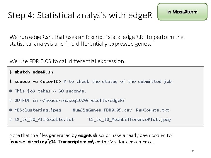
Step 4: Statistical analysis with edge. R In Moba. Xterm We run edge. R. sh, that uses an R script “stats_edge. R. R” to perform the statistical analysis and find differentially expressed genes. We use FDR 0. 05 to call differential expression. $ sbatch edge. R. sh $ squeue –u <user. ID> # to check the status of the submitted job # This job takes ~ 30 seconds. # OUTPUT in ~/mouse-rnaseq 2020/results/edge. R/ # MDSclustering. jpeg Num. Sig. Genes_FDR 0. 05. csv Raw. Counts. txt # t 8_vs_t 0_All. Results. txt t 8_vs_t 0_Mean. Difference. Plot. jpeg Note that the files generated by edge. R. sh script have already been copied to [course_directory]4_Transcriptomics on the VM for convenience. 34

Exit Moba. Xterm by either closing the window or typing ‘exit’ in the command prompt. Genome Assembly | Saba Ghaffari | 2020 36

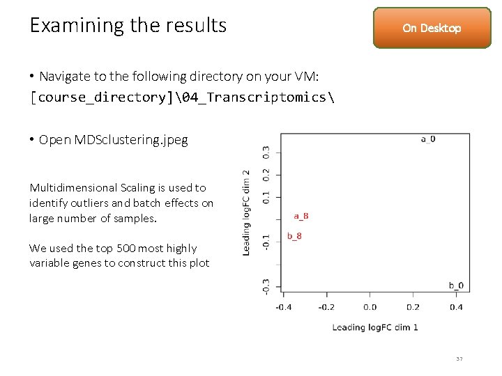
Examining the results On Desktop • Navigate to the following directory on your VM: [course_directory]4_Transcriptomics • Open MDSclustering. jpeg Multidimensional Scaling is used to identify outliers and batch effects on large number of samples. We used the top 500 most highly variable genes to construct this plot 37

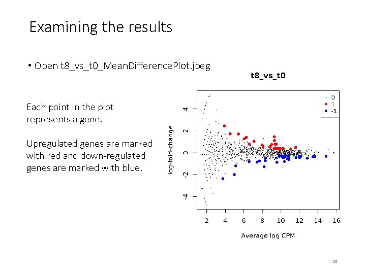
Examining the results • Open t 8_vs_t 0_Mean. Difference. Plot. jpeg Each point in the plot represents a gene. Upregulated genes are marked with red and down-regulated genes are marked with blue. 38

Visualization Using IGV The Integrative Genomics Viewer (IGV) is a tool that supports the visualization of mapped reads to a reference genome, among other functionalities. We will use it to observe where hits were called for the alignment for the two samples (TP 0 and TP 8), and the differentially expressed genes. 39

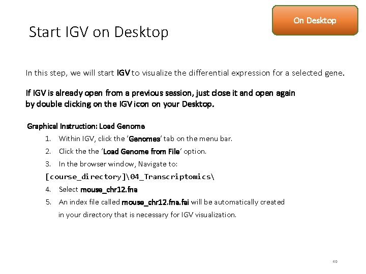
Start IGV on Desktop On Desktop In this step, we will start IGV to visualize the differential expression for a selected gene. If IGV is already open from a previous session, just close it and open again by double clicking on the IGV icon on your Desktop. Graphical Instruction: Load Genome 1. Within IGV, click the ‘Genomes’ tab on the menu bar. 2. Click the ‘Load Genome from File’ option. 3. In the browser window, Navigate to: [course_directory]4_Transcriptomics 4. Select mouse_chr 12. fna 5. An index file called mouse_chr 12. fna. fai will be automatically created in your directory that is necessary for IGV visualization. 40

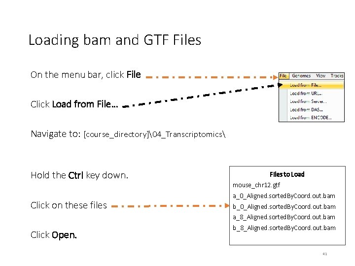
Loading bam and GTF Files On the menu bar, click File Click Load from File… Navigate to: [course_directory]4_Transcriptomics Hold the Ctrl key down. Click on these files Files to Load mouse_chr 12. gtf a_0_Aligned. sorted. By. Coord. out. bam b_0_Aligned. sorted. By. Coord. out. bam a_8_Aligned. sorted. By. Coord. out. bam Click Open. b_8_Aligned. sorted. By. Coord. out. bam 41

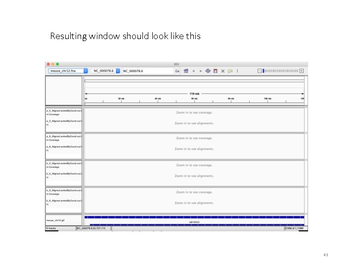
Resulting window should look like this 42

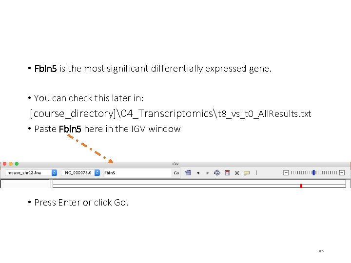
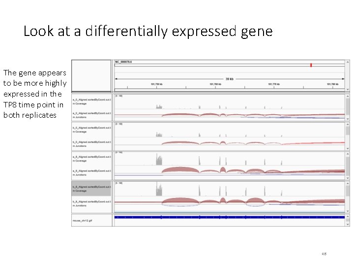
• Fbln 5 is the most significant differentially expressed gene. • You can check this later in: [course_directory]4_Transcriptomicst 8_vs_t 0_All. Results. txt • Paste Fbln 5 here in the IGV window • Press Enter or click Go. 43

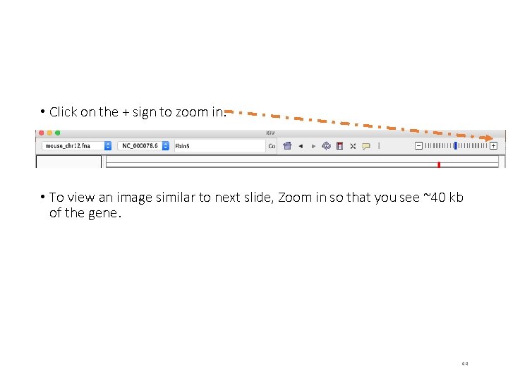
• Click on the + sign to zoom in. • To view an image similar to next slide, Zoom in so that you see ~40 kb of the gene. 44

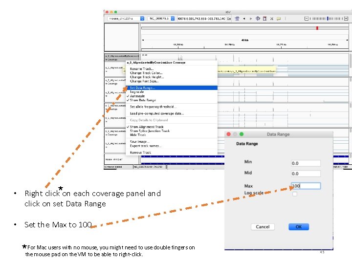
• Right click on each coverage panel and click on set Data Range • Set the Max to 100 For Mac users with no mouse, you might need to use double fingers on the mouse pad on the VM to be able to right-click. 45

Look at a differentially expressed gene The gene appears to be more highly expressed in the TP 8 time point in both replicates 46