Randomized Algorithms William Cohen Outline Randomized methods SGD

Randomized Algorithms William Cohen

Outline • Randomized methods – SGD with the hash trick (review) – Other randomized algorithms • Bloom filters • Locality sensitive hashing

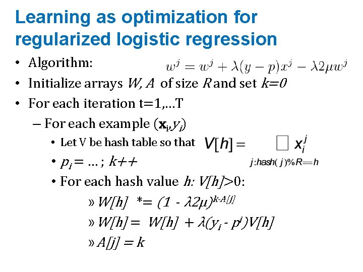
Learning as optimization for regularized logistic regression • Algorithm: • Initialize arrays W, A of size R and set k=0 • For each iteration t=1, …T – For each example (xi, yi) • Let V be hash table so that • pi = … ; k++ • For each hash value h: V[h]>0: » W[h] *= (1 - λ 2μ)k-A[j] » W[h] = W[h] + λ(yi - pi)V[h] » A[j] = k

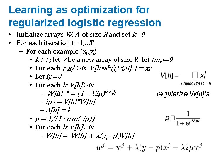
Learning as optimization for regularized logistic regression • Initialize arrays W, A of size R and set k=0 • For each iteration t=1, …T – For each example (xi, yi) • k++; let V be a new array of size R; let tmp=0 • For each j: xi j >0: V[hash(j)%R] += xi j • Let ip=0 • For each h: V[h]>0: – W[h] *= (1 - λ 2μ)k-A[j] regularize W[h]’s – ip+= V[h]*W[h] – A[h] = k • p = 1/(1+exp(-ip)) • For each h: V[h]>0: – W[h] = W[h] + λ(yi - pi)V[h]

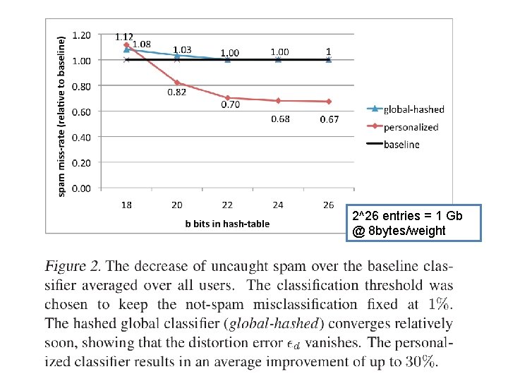
An example 2^26 entries = 1 Gb @ 8 bytes/weight

Results

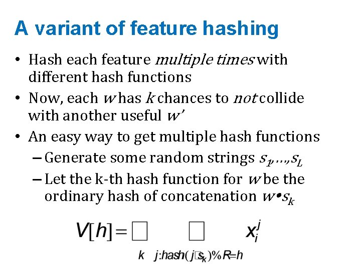
A variant of feature hashing • Hash each feature multiple times with different hash functions • Now, each w has k chances to not collide with another useful w’ • An easy way to get multiple hash functions – Generate some random strings s 1, …, s. L – Let the k-th hash function for w be the ordinary hash of concatenation w sk

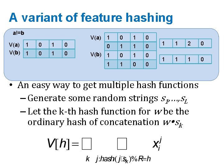
A variant of feature hashing a!=b 1 0 1 times 0 • Hash each feature. V(a) multiple with 1 1 2 0 0 1 0 V(a) 1 0 1 1 0 different hash functions V(b) 1 0 1 0 1 1 1 0 • Now, each w has k chances to not collide 1 1 0 0 with another useful w’ • An easy way to get multiple hash functions – Generate some random strings s 1, …, s. L – Let the k-th hash function for w be the ordinary hash of concatenation w sk

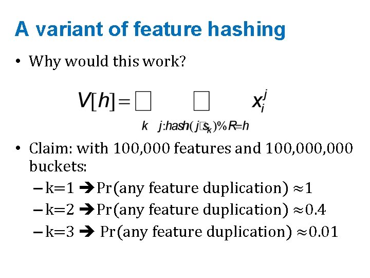
A variant of feature hashing • Why would this work? • Claim: with 100, 000 features and 100, 000 buckets: – k=1 Pr(any feature duplication) ≈1 – k=2 Pr(any feature duplication) ≈0. 4 – k=3 Pr(any feature duplication) ≈0. 01

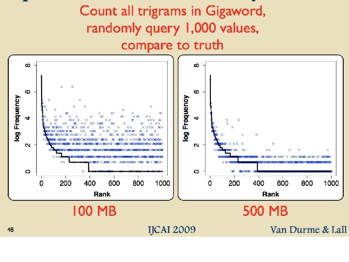
Hash Trick - Insights • Save memory: don’t store hash keys • Allow collisions – even though it distorts your data some • Let the learner (downstream) take up the slack • Here’s another famous trick that exploits these insights….

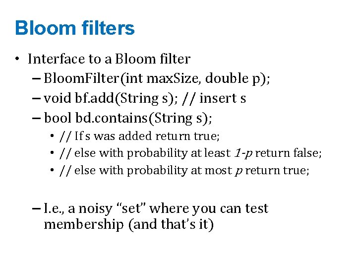
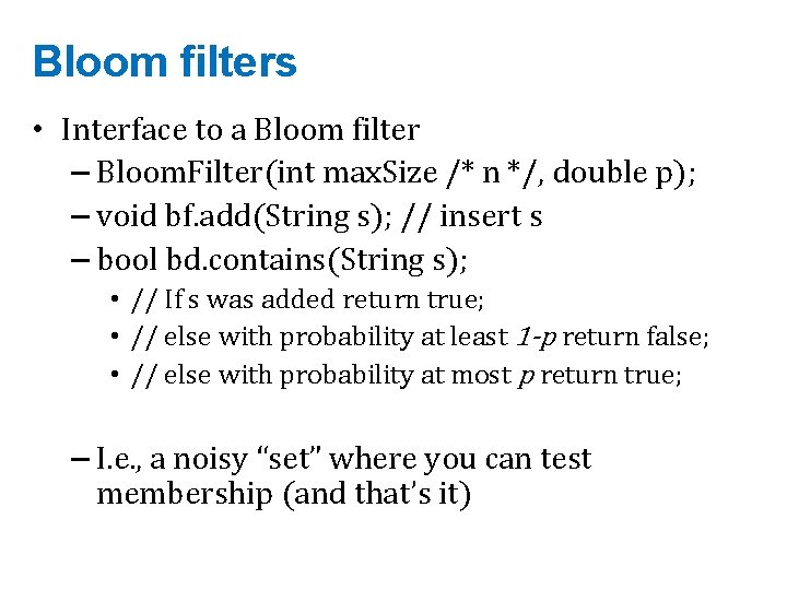
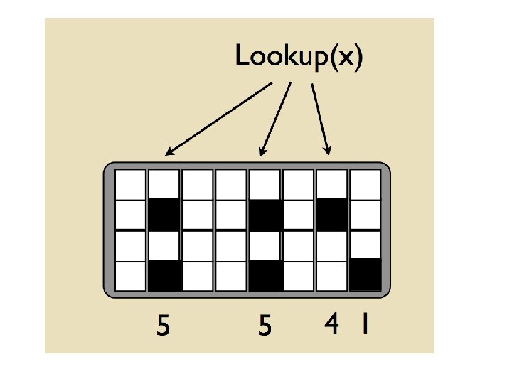
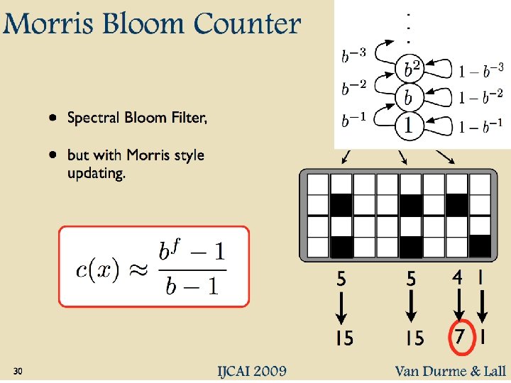
Bloom filters • Interface to a Bloom filter – Bloom. Filter(int max. Size, double p); – void bf. add(String s); // insert s – bool bd. contains(String s); • // If s was added return true; • // else with probability at least 1 -p return false; • // else with probability at most p return true; – I. e. , a noisy “set” where you can test membership (and that’s it)

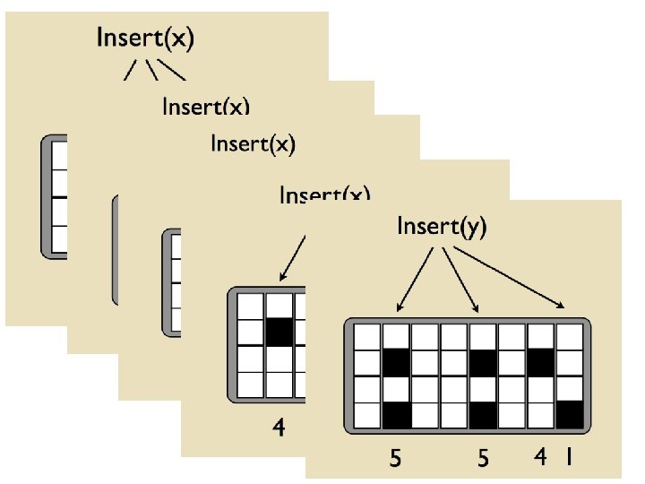
Bloom filters • An implementation – Allocate M bits, bit[0]…, bit[1 -M] – Pick K hash functions hash(1, 2), hash(2, s), …. • E. g: hash(i, s) = hash(s+ random. String[i]) – To add string s: • For i=1 to k, set bit[hash(i, s)] = 1 – To check contains(s): • For i=1 to k, test bit[hash(i, s)] • Return “true” if they’re all set; otherwise, return “false” – We’ll discuss how to set M and K soon, but for now: • Let M = 1. 5*max. Size // less than two bits per item! • Let K = 2*log(1/p) // about right with this M

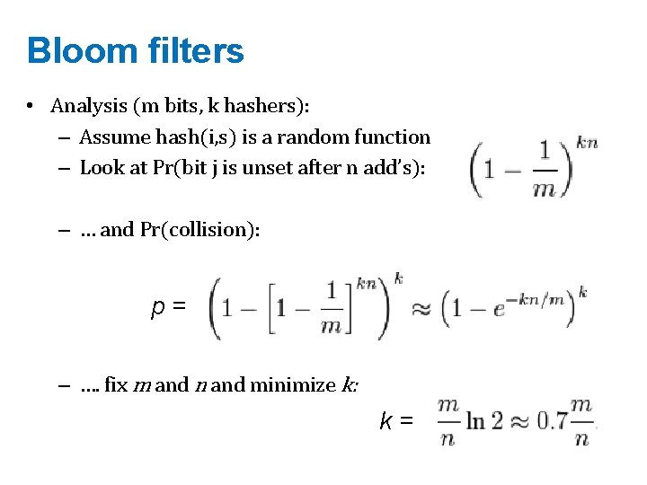
Bloom filters • Analysis (m bits, k hashers): – Assume hash(i, s) is a random function – Look at Pr(bit j is unset after n add’s): – … and Pr(collision): p= – …. fix m and n and minimize k: k=

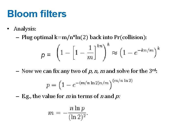
Bloom filters • Analysis: – Plug optimal k=m/n*ln(2) back into Pr(collision): p= – Now we can fix any two of p, n, m and solve for the 3 rd: – E. g. , the value for m in terms of n and p:

Bloom filters • Interface to a Bloom filter – Bloom. Filter(int max. Size /* n */, double p); – void bf. add(String s); // insert s – bool bd. contains(String s); • // If s was added return true; • // else with probability at least 1 -p return false; • // else with probability at most p return true; – I. e. , a noisy “set” where you can test membership (and that’s it)

Bloom filters: demo

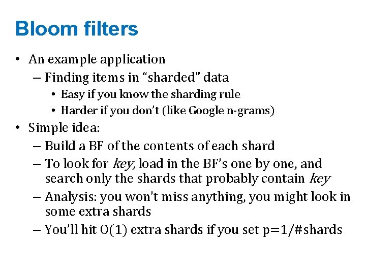
Bloom filters • An example application – Finding items in “sharded” data • Easy if you know the sharding rule • Harder if you don’t (like Google n-grams) • Simple idea: – Build a BF of the contents of each shard – To look for key, load in the BF’s one by one, and search only the shards that probably contain key – Analysis: you won’t miss anything, you might look in some extra shards – You’ll hit O(1) extra shards if you set p=1/#shards

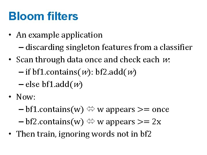
Bloom filters • An example application – discarding singleton features from a classifier • Scan through data once and check each w: – if bf 1. contains(w): bf 2. add(w) – else bf 1. add(w) • Now: – bf 1. contains(w) w appears >= once – bf 2. contains(w) w appears >= 2 x • Then train, ignoring words not in bf 2

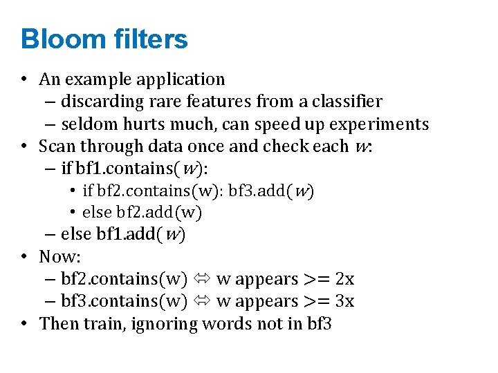
Bloom filters • An example application – discarding rare features from a classifier – seldom hurts much, can speed up experiments • Scan through data once and check each w: – if bf 1. contains(w): • if bf 2. contains(w): bf 3. add(w) • else bf 2. add(w) – else bf 1. add(w) • Now: – bf 2. contains(w) w appears >= 2 x – bf 3. contains(w) w appears >= 3 x • Then train, ignoring words not in bf 3

Locality Sensitive Hashing (LSH)

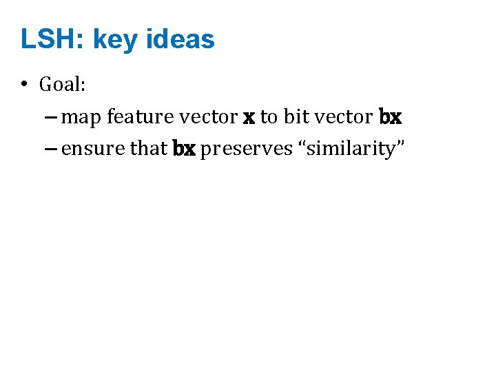
LSH: key ideas • Goal: – map feature vector x to bit vector bx – ensure that bx preserves “similarity”

Random Projections

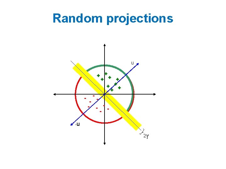
Random projections u + ++ + - -- - - -u 2γ

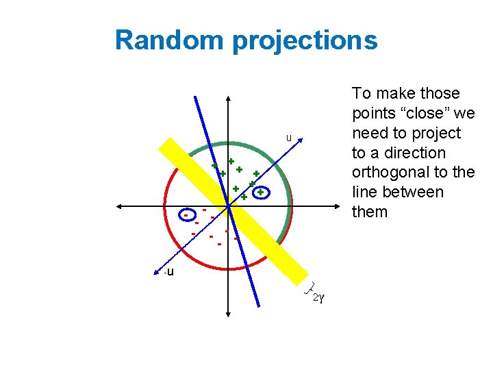
Random projections To make those points “close” we need to project to a direction orthogonal to the line between them u + ++ + - -- - - -u 2γ

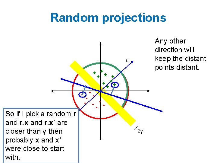
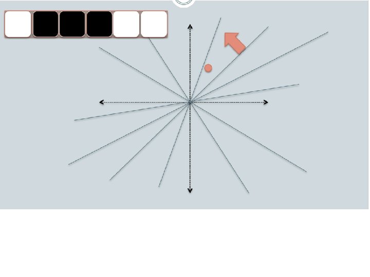
Random projections Any other direction will keep the distant points distant. u + ++ + - -- - So if I pick a random r and r. x’ are -u closer than γ then probably x and x’ were close to start with. 2γ

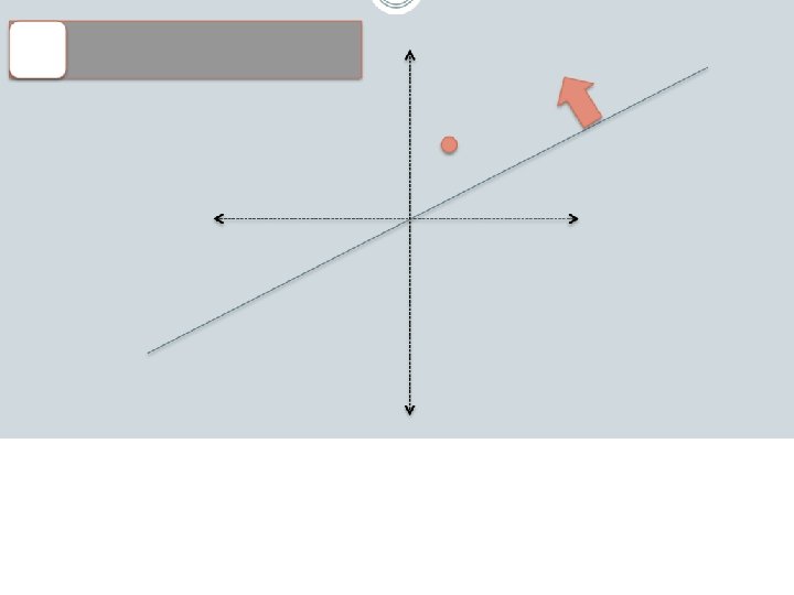
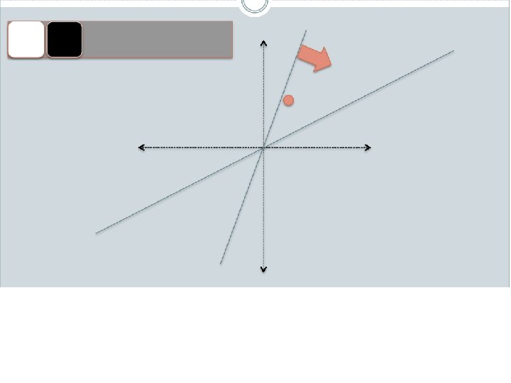
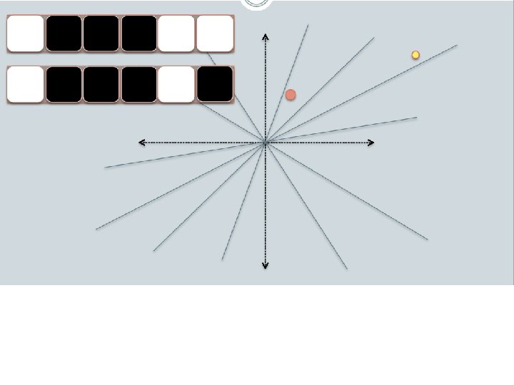
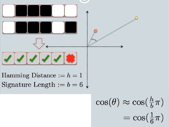
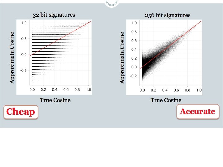
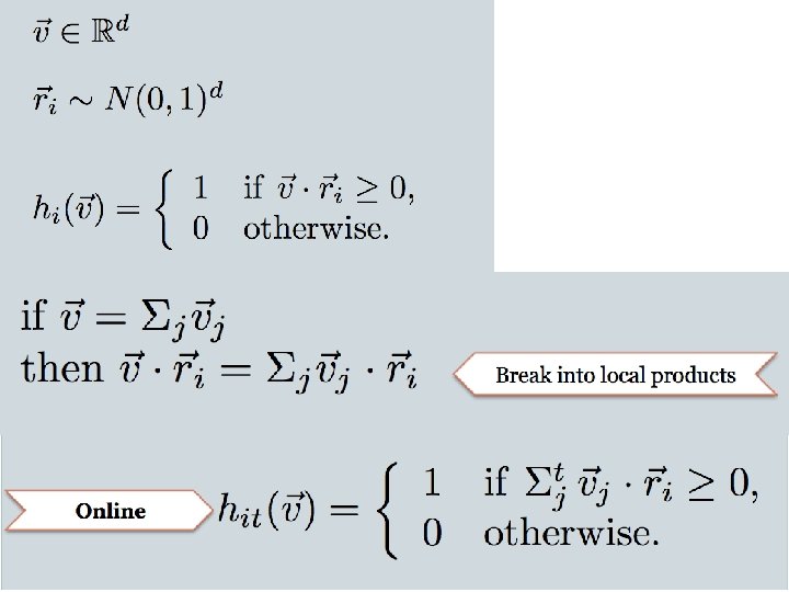
LSH: key ideas • Goal: – map feature vector x to bit vector bx – ensure that bx preserves “similarity” • Basic idea: use random projections of x – Repeat many times: • Pick a random hyperplane r • Compute the inner product of r with x • Record if x is “close to” r (r. x>=0) – the next bit in bx • Theory says that is x’ and x have small cosine distance then bx and bx’ will have small Hamming distance

LSH: key ideas • Naïve algorithm: – Initialization: • For i=1 to output. Bits: – For each feature f: » Draw r(f, i) ~ Normal(0, 1) – Given an instance x • For i=1 to output. Bits: LSH[i] = sum(x[f]*r[i, f] for f with non-zero weight in x) > 0 ? 1 : 0 • Return the bit-vector LSH – Problem: • the array of r’s is very large

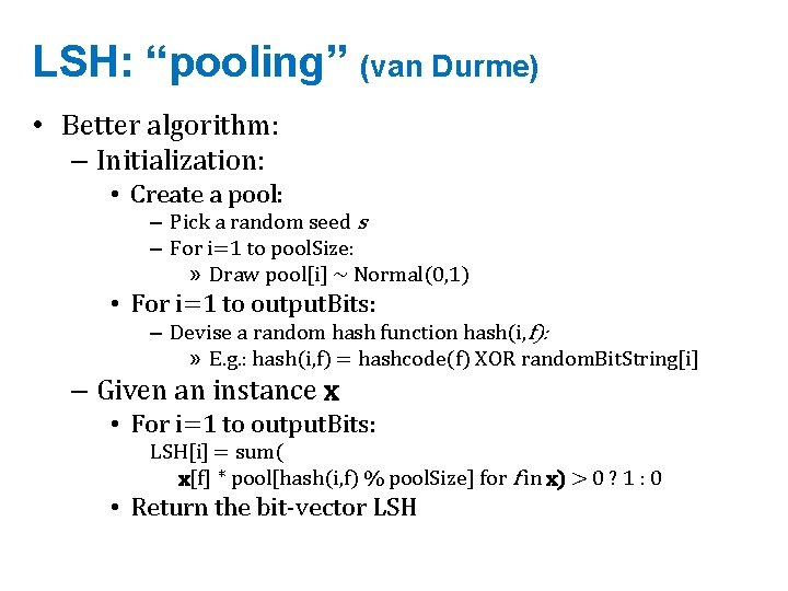
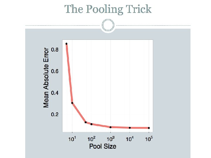
LSH: “pooling” (van Durme) • Better algorithm: – Initialization: • Create a pool: – Pick a random seed s – For i=1 to pool. Size: » Draw pool[i] ~ Normal(0, 1) • For i=1 to output. Bits: – Devise a random hash function hash(i, f): » E. g. : hash(i, f) = hashcode(f) XOR random. Bit. String[i] – Given an instance x • For i=1 to output. Bits: LSH[i] = sum( x[f] * pool[hash(i, f) % pool. Size] for f in x) > 0 ? 1 : 0 • Return the bit-vector LSH

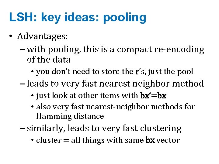
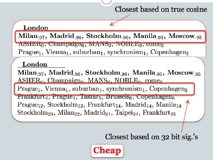
LSH: key ideas: pooling • Advantages: – with pooling, this is a compact re-encoding of the data • you don’t need to store the r’s, just the pool – leads to very fast nearest neighbor method • just look at other items with bx’=bx • also very fast nearest-neighbor methods for Hamming distance – similarly, leads to very fast clustering • cluster = all things with same bx vector

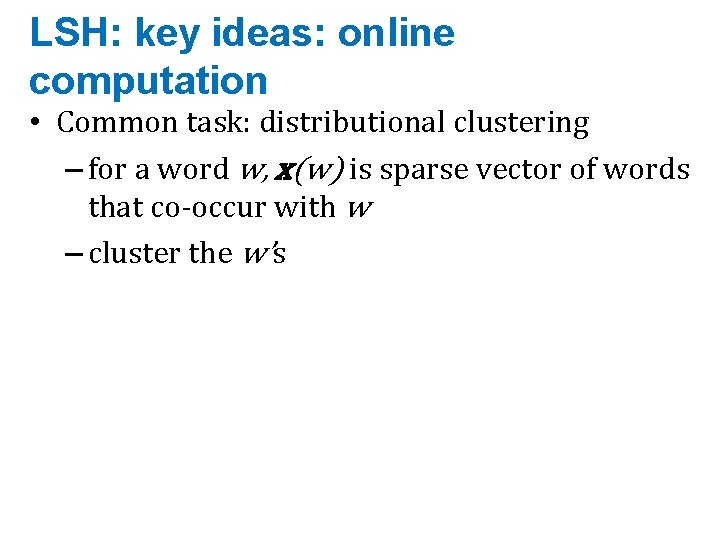
LSH: key ideas: online computation • Common task: distributional clustering – for a word w, x(w) is sparse vector of words that co-occur with w – cluster the w’s

GRAPH ALGORITHMS

Graph algorithms • Page. Rank implementations – in memory – streaming, node list in memory – streaming, no memory – map-reduce • A little like Naïve Bayes variants – data in memory – word counts in memory – stream-and-sort – map-reduce

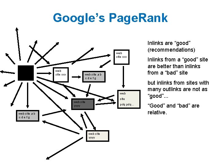
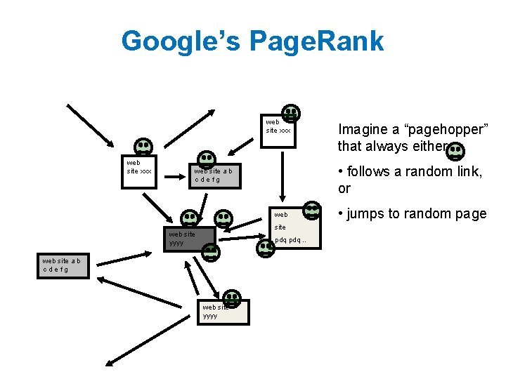
Google’s Page. Rank web site xxx web site a b cdefg web site yyyy pdq. . web site a b cdefg web site yyyy Inlinks are “good” (recommendations) Inlinks from a “good” site are better than inlinks from a “bad” site but inlinks from sites with many outlinks are not as “good”. . . “Good” and “bad” are relative.

Google’s Page. Rank web site xxx • follows a random link, or web site a b cdefg web site yyyy pdq. . web site a b cdefg web site yyyy Imagine a “pagehopper” that always either • jumps to random page

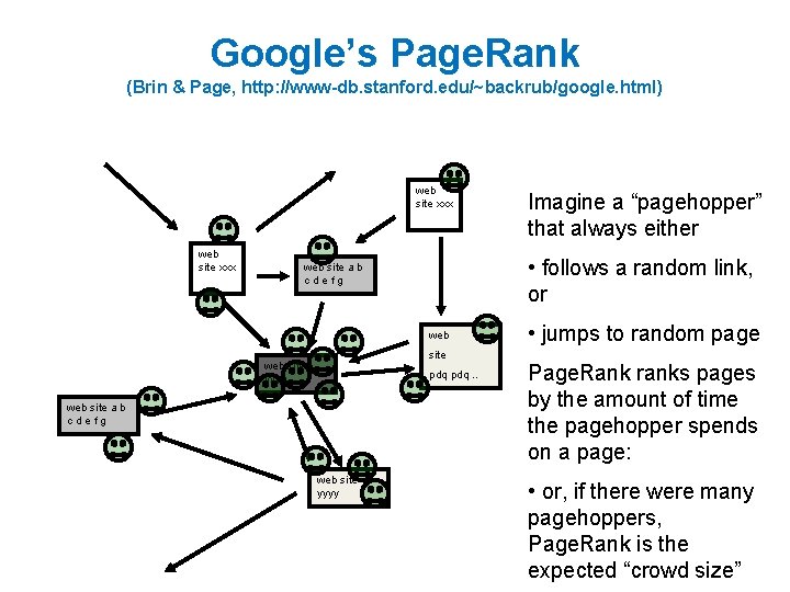
Google’s Page. Rank (Brin & Page, http: //www-db. stanford. edu/~backrub/google. html) web site xxx • follows a random link, or web site a b cdefg web site yyyy pdq. . web site a b cdefg web site yyyy Imagine a “pagehopper” that always either • jumps to random page Page. Rank ranks pages by the amount of time the pagehopper spends on a page: • or, if there were many pagehoppers, Page. Rank is the expected “crowd size”

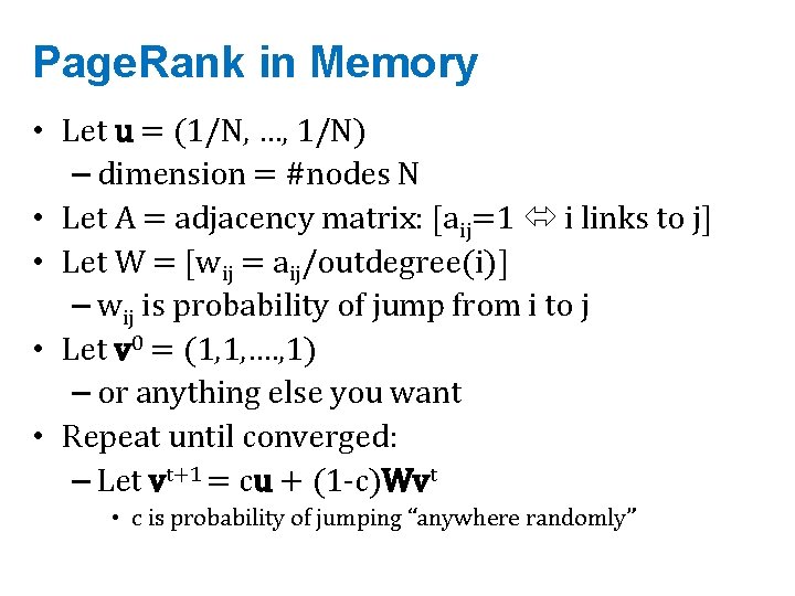
Page. Rank in Memory • Let u = (1/N, …, 1/N) – dimension = #nodes N • Let A = adjacency matrix: [aij=1 i links to j] • Let W = [wij = aij/outdegree(i)] – wij is probability of jump from i to j • Let v 0 = (1, 1, …. , 1) – or anything else you want • Repeat until converged: – Let vt+1 = cu + (1 -c)Wvt • c is probability of jumping “anywhere randomly”

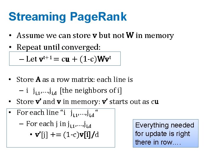
Streaming Page. Rank • Assume we can store v but not W in memory • Repeat until converged: – Let vt+1 = cu + (1 -c)Wvt • Store A as a row matrix: each line is – i ji, 1, …, ji, d [the neighbors of i] • Store v’ and v in memory: v’ starts out as cu • For each line “i ji, 1, …, ji, d “ – For each j in ji, 1, …, ji, d Everything needed for update is right • v’[j] += (1 -c)v[i]/d there in row….

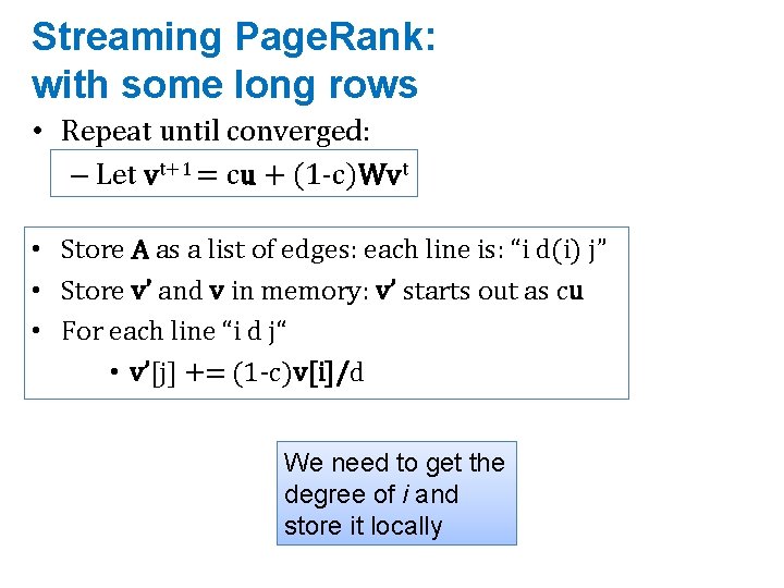
Streaming Page. Rank: with some long rows • Repeat until converged: – Let vt+1 = cu + (1 -c)Wvt • Store A as a list of edges: each line is: “i d(i) j” • Store v’ and v in memory: v’ starts out as cu • For each line “i d j“ • v’[j] += (1 -c)v[i]/d We need to get the degree of i and store it locally

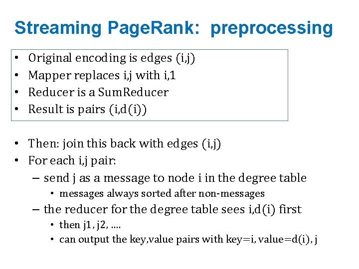
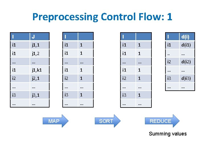
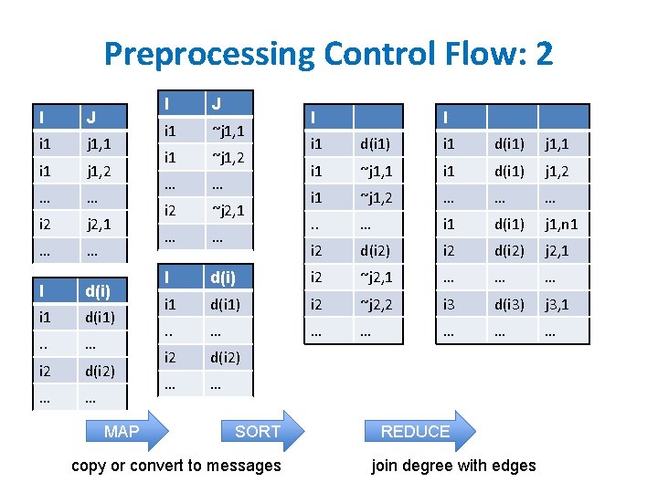
Streaming Page. Rank: preprocessing • • Original encoding is edges (i, j) Mapper replaces i, j with i, 1 Reducer is a Sum. Reducer Result is pairs (i, d(i)) • Then: join this back with edges (i, j) • For each i, j pair: – send j as a message to node i in the degree table • messages always sorted after non-messages – the reducer for the degree table sees i, d(i) first • then j 1, j 2, …. • can output the key, value pairs with key=i, value=d(i), j

Preprocessing Control Flow: 1 I J I i 1 j 1, 1 i 1 i 1 j 1, 2 i 1 1 … … … i 1 j 1, k 1 i 2 I d(i) 1 i 1 d(i 1) i 1 1 . . … … i 2 d(i 2) i 1 1 … … j 2, 1 i 2 1 i 3 d)i 3) … … … … i 3 j 3, 1 i 3 1 … … … MAP I SORT REDUCE Summing values

Preprocessing Control Flow: 2 I J i 1 j 1, 1 i 1 j 1, 2 … … i 2 j 2, 1 … … I d(i) i 1 d(i 1) . . … i 2 d(i 2) … … MAP I J i 1 ~j 1, 1 i 1 ~j 1, 2 … … i 2 ~j 2, 1 … … I I I i 1 d(i 1) j 1, 1 i 1 ~j 1, 1 i 1 d(i 1) j 1, 2 i 1 ~j 1, 2 … … … . . … i 1 d(i 1) j 1, n 1 i 2 d(i 2) j 2, 1 d(i) i 2 ~j 2, 1 … … … i 1 d(i 1) i 2 ~j 2, 2 i 3 d(i 3) j 3, 1 . . … … … i 2 d(i 2) … … SORT copy or convert to messages REDUCE join degree with edges

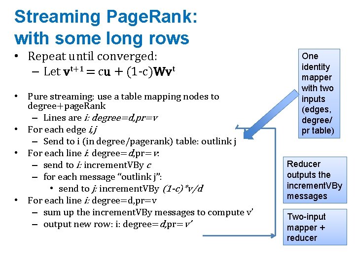
Streaming Page. Rank: with some long rows • Repeat until converged: – Let vt+1 = cu + (1 -c)Wvt • Pure streaming: use a table mapping nodes to degree+page. Rank – Lines are i: degree=d, pr=v • For each edge i, j – Send to i (in degree/pagerank) table: outlink j • For each line i: degree=d, pr=v: – send to i: increment. VBy c – for each message “outlink j”: • send to j: increment. VBy (1 -c)*v/d • For each line i: degree=d, pr=v – sum up the increment. VBy messages to compute v’ – output new row: i: degree=d, pr=v’ One identity mapper with two inputs (edges, degree/ pr table) Reducer outputs the increment. VBy messages Two-input mapper + reducer

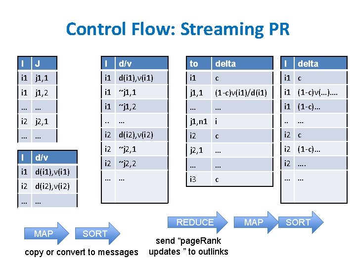
Control Flow: Streaming PR I J I d/v to delta I delta i 1 j 1, 1 i 1 d(i 1), v(i 1) i 1 c i 1 j 1, 2 i 1 ~j 1, 1 (1 -c)v(i 1)/d(i 1) i 1 (1 -c)v(…)…. … … i 1 ~j 1, 2 … … i 1 (1 -c)… i 2 j 2, 1 . . j 1, n 1 i . . … … i 2 d(i 2), v(i 2) i 2 c i 2 ~j 2, 1 … i 2 (1 -c)… i 2 ~j 2, 2 … … i 2 …. … … i 3 c … … I d/v i 1 d(i 1), v(i 1) i 2 d(i 2), v(i 2) … … REDUCE MAP SORT copy or convert to messages send “page. Rank updates ” to outlinks MAP SORT

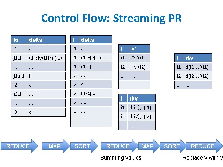
Control Flow: Streaming PR to delta I delta i 1 c I v’ j 1, 1 (1 -c)v(i 1)/d(i 1) i 1 (1 -c)v(…)…. i 1 ~v’(i 1) I … … i 1 (1 -c)… i 2 ~v’(i 2) i 1 d(i 1), v’(i 1) j 1, n 1 i . . … … i 2 d(i 2), v’(i 2) i 2 c j 2, 1 … i 2 (1 -c)… … … i 2 …. i 3 c … … … d/v … … I d/v i 1 d(i 1), v(i 1) i 2 d(i 2), v(i 2) … … REDUCE MAP SORT REDUCE MAP Summing values SORT REDUCE Replace v with v’

Control Flow: Streaming PR I J i 1 j 1, 1 i 1 j 1, 2 … … i 2 j 2, 1 … … I d/v i 1 d(i 1), v(i 1) i 2 d(i 2), v(i 2) … … MAP copy or convert to messages and back around for next iteration….

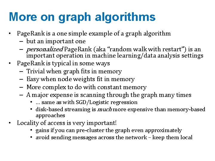
More on graph algorithms • Page. Rank is a one simple example of a graph algorithm – but an important one – personalized Page. Rank (aka “random walk with restart”) is an important operation in machine learning/data analysis settings • Page. Rank is typical in some ways – Trivial when graph fits in memory – Easy when node weights fit in memory – More complex to do with constant memory – A major expense is scanning through the graph many times • … same as with SGD/Logistic regression • disk-based streaming is much more expensive than memory-based approaches • Locality of access is very important! • gains if you can pre-cluster the graph even approximately • avoid sending messages across the network – keep them local

Machine Learning in Graphs - 2010

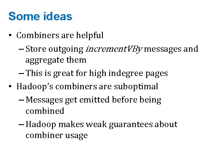
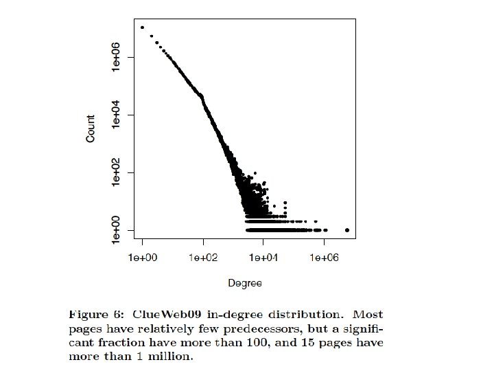
Some ideas • Combiners are helpful – Store outgoing increment. VBy messages and aggregate them – This is great for high indegree pages • Hadoop’s combiners are suboptimal – Messages get emitted before being combined – Hadoop makes weak guarantees about combiner usage

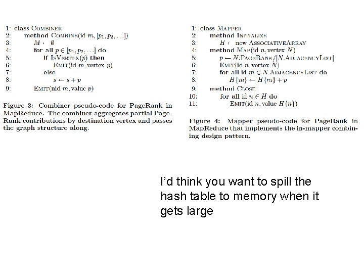
I’d think you want to spill the hash table to memory when it gets large

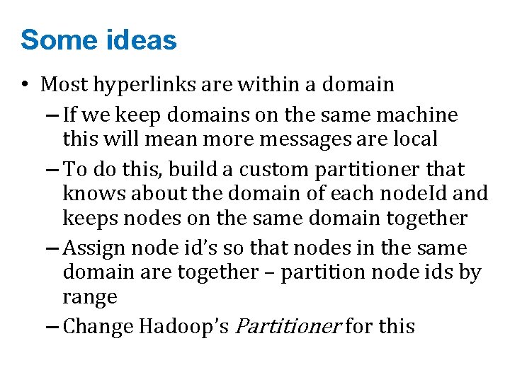
Some ideas • Most hyperlinks are within a domain – If we keep domains on the same machine this will mean more messages are local – To do this, build a custom partitioner that knows about the domain of each node. Id and keeps nodes on the same domain together – Assign node id’s so that nodes in the same domain are together – partition node ids by range – Change Hadoop’s Partitioner for this

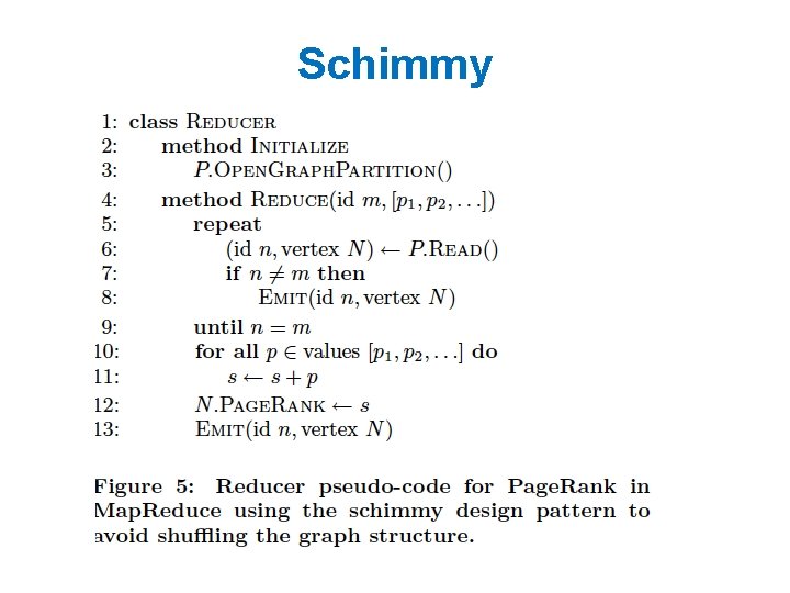
Some ideas • Repeatedly shuffling the graph is expensive – We should separate the messages about the graph structure (fixed over time) from messages about page. Rank weights (variable) – compute and distribute the edges once – read them in incrementally in the reducer • not easy to do in Hadoop! – call this the “Schimmy” pattern

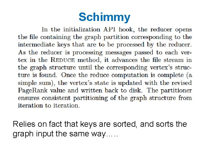
Schimmy Relies on fact that keys are sorted, and sorts the graph input the same way…. .

Schimmy